Sara A. Stoudt, PhD: Troubles with Tibble

require(readr)
require(dplyr)
require(ggplot2)
require(tibble)
require(data.table)
require(gridExtra)

Note: I’m skipping over purrr until @kellieotto returns from her travels, so we can write our joint post.

This week’s post is on tibbles. This actually came at a perfect time since recently I’ve run into a few mysteries where I get unexpected errors or output after a data frame gets turned into a tibble at some point during my workflow (like when I use functions from the tidyverse). This is actually a good sign because it means I’m using the tidyverse more in my day to day work. So now to solve some tibble troubles.

Mystery #1

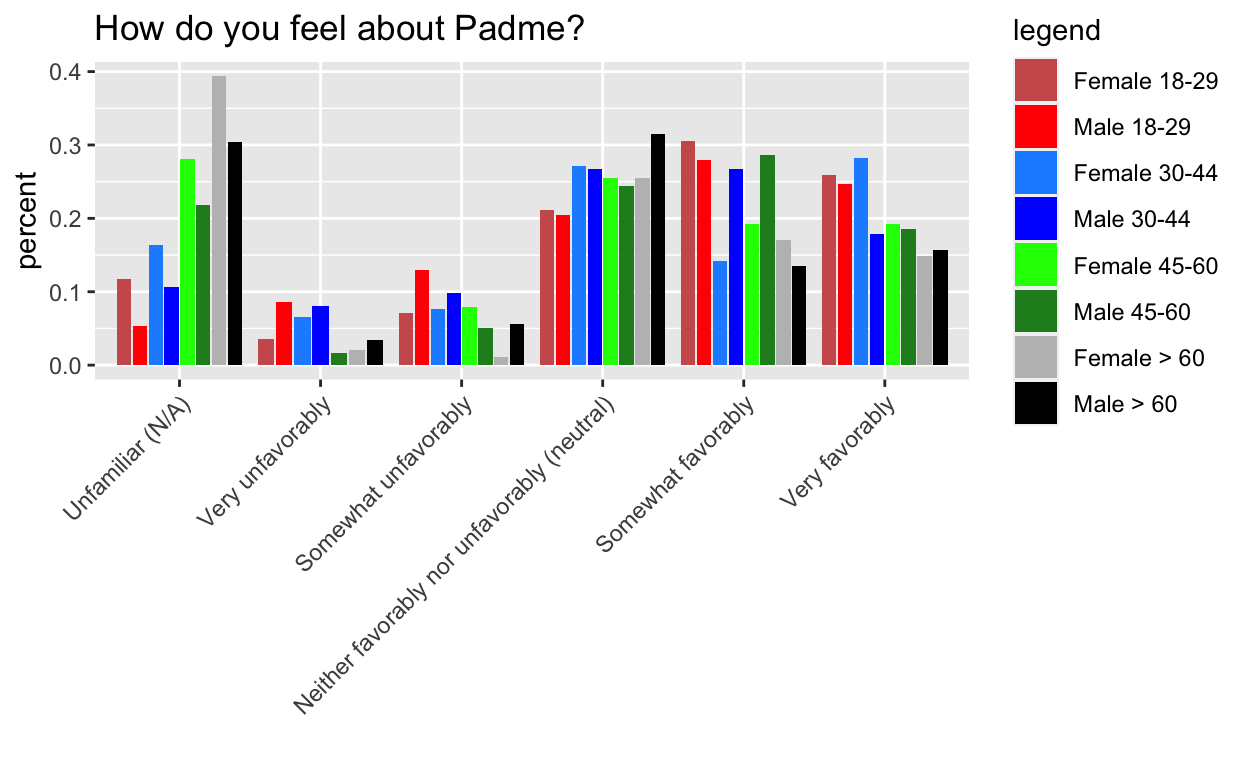
This mystery comes from Week 7 of Tidy Tuesday, the dreaded barplots. I’m hiding the process code to streamline the post, but if you want to see it, go here. The gist of it, is that I want the order of the side by side bars to be consistent within category.

The key is to pre-arrange the data to follow the order that we want to plot it in.

g1 doesn’t work, but g2, g3, and g4 do.

Key: It turns out that the tibble format isn’t the issue per se, it is tibble’s lazy evaluation (and ggplot’s) that is the real issue. This is analogous to why you need aes_string instead of aes when you are passing in a variable name to ggplot in a custom made function. The rearranging doesn’t actually happen until wrapped in another function that evaulates it.

toPlot

# A tibble: 47 x 7
# Groups:   Gender, Age [8]
   Gender Age   V28                 count.x count.y percent genderAge 
   <fct>  <fct> <fct>                 <int>   <int>   <dbl> <fct>     
 1 Female > 60  Unfamiliar (N/A)         37      94  0.394  Female > …
 2 Female > 60  Very unfavorably          2      94  0.0213 Female > …
 3 Female > 60  Somewhat unfavorab…       1      94  0.0106 Female > …
 4 Female > 60  Neither favorably …      24      94  0.255  Female > …
 5 Female > 60  Somewhat favorably       16      94  0.170  Female > …
 6 Female > 60  Very favorably           14      94  0.149  Female > …
 7 Female 18-29 Unfamiliar (N/A)         10      85  0.118  Female 18…
 8 Female 18-29 Very unfavorably          3      85  0.0353 Female 18…
 9 Female 18-29 Somewhat unfavorab…       6      85  0.0706 Female 18…
10 Female 18-29 Neither favorably …      18      85  0.212  Female 18…
# … with 37 more rows

test <- toPlot %>% arrange(Age, V28)
is.tibble(test)

[1] TRUE

test2 <- as.data.frame(toPlot %>% arrange(Age, V28))
test3 <- data.frame(toPlot %>% arrange(Age, V28))
test4 <- as.tibble(toPlot %>% arrange(Age, V28))
# test5=tibble(toPlot%>%arrange(Age,V28)) ## Error: Column `toPlot %>% arrange(Age, V28)` must be a 1d atomic vector or a list


g1 <- ggplot(test, aes(V28, y = percent, fill = genderAge)) +
  geom_bar(stat = "identity", position = position_dodge2(preserve = "total")) +
  theme(axis.text.x = element_text(angle = 45, hjust = 1)) +
  xlab("") +
  ggtitle("How do you feel about Padme?") +
  scale_fill_manual("legend", values = c("Female 18-29" = "indianred", "Male 18-29" = "red", "Female 30-44" = "dodgerblue", "Male 30-44" = "blue", "Female 45-60" = "green", "Male 45-60" = "forestgreen", "Female > 60" = "grey", "Male > 60" = "black"))


g2 <- ggplot(test2, aes(V28, y = percent, fill = genderAge)) +
  geom_bar(stat = "identity", position = position_dodge2(preserve = "total")) +
  theme(axis.text.x = element_text(angle = 45, hjust = 1)) +
  xlab("") +
  ggtitle("How do you feel about Padme?") +
  scale_fill_manual("legend", values = c("Female 18-29" = "indianred", "Male 18-29" = "red", "Female 30-44" = "dodgerblue", "Male 30-44" = "blue", "Female 45-60" = "green", "Male 45-60" = "forestgreen", "Female > 60" = "grey", "Male > 60" = "black"))

g3 <- ggplot(test3, aes(V28, y = percent, fill = genderAge)) +
  geom_bar(stat = "identity", position = position_dodge2(preserve = "total")) +
  theme(axis.text.x = element_text(angle = 45, hjust = 1)) +
  xlab("") +
  ggtitle("How do you feel about Padme?") +
  scale_fill_manual("legend", values = c("Female 18-29" = "indianred", "Male 18-29" = "red", "Female 30-44" = "dodgerblue", "Male 30-44" = "blue", "Female 45-60" = "green", "Male 45-60" = "forestgreen", "Female > 60" = "grey", "Male > 60" = "black"))

g4 <- ggplot(test4, aes(V28, y = percent, fill = genderAge)) +
  geom_bar(stat = "identity", position = position_dodge2(preserve = "total")) +
  theme(axis.text.x = element_text(angle = 45, hjust = 1)) +
  xlab("") +
  ggtitle("How do you feel about Padme?") +
  scale_fill_manual("legend", values = c("Female 18-29" = "indianred", "Male 18-29" = "red", "Female 30-44" = "dodgerblue", "Male 30-44" = "blue", "Female 45-60" = "green", "Male 45-60" = "forestgreen", "Female > 60" = "grey", "Male > 60" = "black"))


g1

g2

g3

g4

Mystery #2

This mystery comes from a scenario at work. I had one dataset that had different states than another dataset (state was treated as a factor). I wanted to find new levels and replace them with a catch all “other” level. I started with a data frame, but I used complete from tidyr at some point, and unknowingly had switched to a tibble. Therefore, my subsetting procedure was not doing what I expected. Here is a simplified example:

state <- tibble(state = as.factor(c("AL", "AK", "AR", "AS")))
state2 <- tibble(state = as.factor(c("AL", "AK", "AR", "AS", "CA", "CO")))

What I did:

state2[, 1] %in% levels(state[, 1])

[1] FALSE

levels(state[, 1])

NULL

What I should have did given that I’m working with tibbles:

test <- state2[[1]] %in% levels(state[[1]])
test

[1]  TRUE  TRUE  TRUE  TRUE FALSE FALSE

Key: subsetting tibbles by column requires the double brackets

What I did:

state2[, 1] <- as.character(state2[, 1])
state2

# A tibble: 6 x 1
  state              
  <chr>              
1 c(2, 1, 3, 4, 5, 6)
2 c(2, 1, 3, 4, 5, 6)
3 c(2, 1, 3, 4, 5, 6)
4 c(2, 1, 3, 4, 5, 6)
5 c(2, 1, 3, 4, 5, 6)
6 c(2, 1, 3, 4, 5, 6)

What I should have did given that I’m working with tibbles:

Key: again this is a subsetting syntax issue

state2 <- tibble(state = as.factor(c("AL", "AK", "AR", "AS", "CA", "CO")))

state2[[1]] <- as.character(state2[[1]])
state2[test, 1] <- "other"

Compare to behavior on a dataframe (this is the output I expected):

state <- data.frame(state = as.factor(c("AL", "AK", "AR", "AS")))
state2 <- data.frame(state = as.factor(c("AL", "AK", "AR", "AS", "CA", "CO")))

state2[, 1] %in% levels(state[, 1])

[1]  TRUE  TRUE  TRUE  TRUE FALSE FALSE

levels(state[, 1])

[1] "AK" "AL" "AR" "AS"

state2[, 1] <- as.character(state2[, 1])
state2

  state
1    AL
2    AK
3    AR
4    AS
5    CA
6    CO

state2[test, 1] <- "other"
state2

  state
1 other
2 other
3 other
4 other
5    CA
6    CO

state2

  state
1 other
2 other
3 other
4 other
5    CA
6    CO

Mystery #3

This mystery comes from my readr post where I wanted to remove rows that had NAs in certain columns and a certain number of characters in another example. Here is a simplified example:

tb <- tibble(x = c(NA, NA, 3), y = c(NA, 2, 1), z = c("A", "BC", "D"))
tb[, 1] ## tibble

# A tibble: 3 x 1
      x
  <dbl>
1    NA
2    NA
3     3

tb[[1]] ## vector

[1] NA NA  3

The difference in subsetting syntax is a reoccurring issue. I use the syntax expecting my data to be a dataframe, but I forgot that tidyverse functions switch to tibbles.

tb[-which(is.na(tb[, 2]) & is.na(tb[, 1]) & nchar(tb[, 3]) <= 1), ]

# A tibble: 0 x 3
# … with 3 variables: x <dbl>, y <dbl>, z <chr>

Weird! I expected the output to remove the first row. What’s going on?

is.na(tb[, 2])

         y
[1,]  TRUE
[2,] FALSE
[3,] FALSE

is.na(tb[, 1])

         x
[1,]  TRUE
[2,]  TRUE
[3,] FALSE

These are fine.

nchar(tb[, 3]) <= 1

    z 
FALSE

nchar(tb[, 3])

 z 
17

Ah, here is the culprit! Switching to tibble subsetting syntax…

nchar(tb[[3]]) <= 1

[1]  TRUE FALSE  TRUE

Much better.

Original:

is.na(tb[, 2]) & is.na(tb[, 1]) & nchar(tb[, 3]) <= 1

         y
[1,] FALSE
[2,] FALSE
[3,] FALSE

Fix:

is.na(tb[, 2]) & is.na(tb[, 1]) & nchar(tb[[3]]) <= 1

         y
[1,]  TRUE
[2,] FALSE
[3,] FALSE

tb[-which(is.na(tb[, 2]) & is.na(tb[, 1]) & nchar(tb[[3]]) <= 1), ]

# A tibble: 2 x 3
      x     y z    
  <dbl> <dbl> <chr>
1    NA     2 BC   
2     3     1 D

Compare to behavior on a dataframe:

tb <- tibble(x = c(NA, NA, 3), y = c(NA, 2, 1), z = c("A", "BC", "D"))
tb2 <- as.data.frame(tb)

tb2[-which(is.na(tb2[, 2]) & is.na(tb2[, 1]) & nchar(tb2[, 3]) <= 1), ]

   x y  z
2 NA 2 BC
3  3 1  D

This is the output I expected.

is.na(tb2[, 2])

[1]  TRUE FALSE FALSE

is.na(tb2[, 1])

[1]  TRUE  TRUE FALSE

nchar(tb2[, 3]) <= 1

[1]  TRUE FALSE  TRUE

The double bracket subsetting also works:

is.na(tb2[[2]])

[1]  TRUE FALSE FALSE

is.na(tb2[[1]])

[1]  TRUE  TRUE FALSE

nchar(tb2[[3]]) <= 1

[1]  TRUE FALSE  TRUE

is.na(tb2[, 2]) & is.na(tb2[, 1]) & nchar(tb2[, 3]) <= 1

[1]  TRUE FALSE FALSE

is.na(tb2[[2]]) & is.na(tb2[[1]]) & nchar(tb2[[3]]) <= 1

[1]  TRUE FALSE FALSE

Take-Away: The unexpected behavior that led to most of these mysteries turned out to be because I was using the wrong subsetting syntax.

Since the double bracket subsetting works for dataframes and tibbles, I should transition to using this syntax so that I am not surprised by output when a tibble gets thrown into the mix.

Resources (these helped me solve my mysteries):

Troubles with Tibble

Mystery #1

Mystery #2

Mystery #3

Feedback, questions, comments, etc. are welcome (@sastoudt).