We are hearing these names a lot, and it’s only going to continue (p.s. VOTE). But don’t these names seem a bit… ordinary to you?
How popular are these Democratic candidate names throughout history? The babynames dataset can help shed some light on this question. Let’s look at the proportion of babies with these particular names over time.
candidates <- c("Elizabeth", "Amy", "Joseph", "Peter", "Bernard", "Michael", "Thomas")
candidate_status <- c(T, F, T, F, T, T, F)

yearTotals <- babynames %>%
  group_by(year) %>%
  summarise(yearTotal = sum(n))

candidateData <- babynames %>%
  filter(name %in% candidates) %>%
  group_by(year, name) %>%
  summarise(count = sum(n))

candidateData <- merge(candidateData, yearTotals, by.x = "year", by.y = "year")
candidateData$prop <- candidateData$count / candidateData$yearTotal


ggplot(candidateData, aes(year, prop, col = name, group = name)) +
  geom_point() +
  geom_line() +
  theme_minimal() +
  ylab("proportion of babies in year")
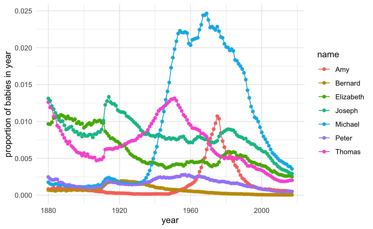
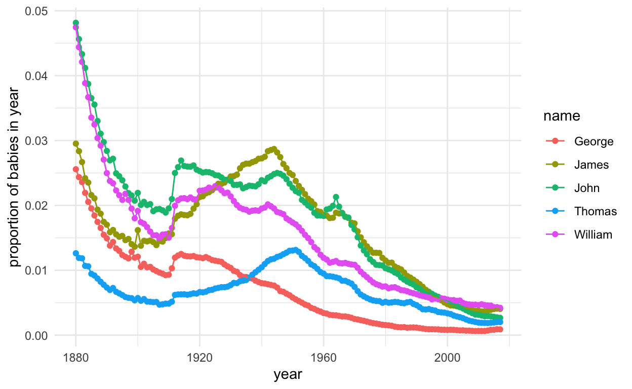
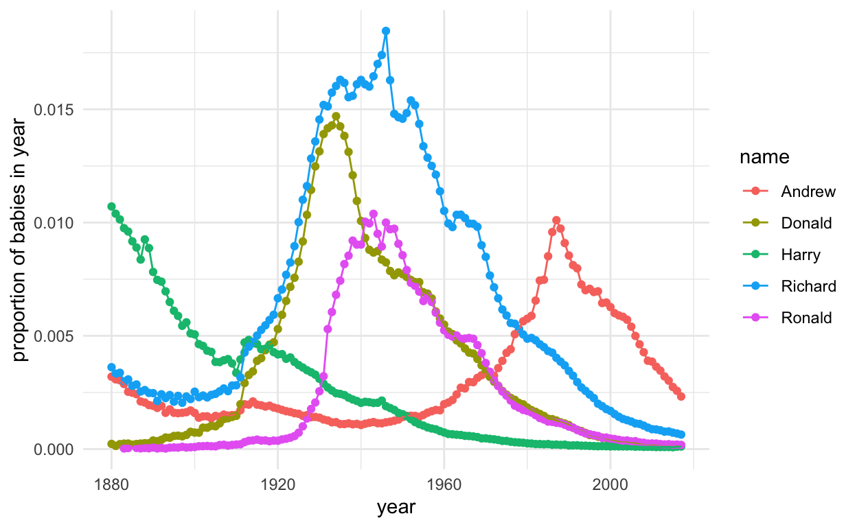
Fad names (with peaks): Amy, Thomas, Michael
More stable names: Bernard, Elizabeth, Joseph, Peter
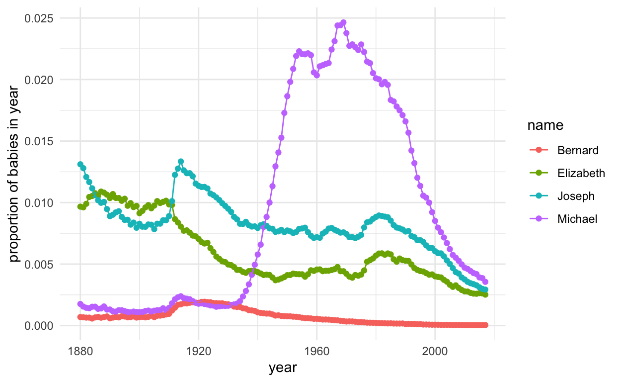
For the sticklers, we can just look at the ones moving forward.
ggplot(subset(candidateData, name %in% candidates[candidate_status]), aes(year, prop, col = name, group = name)) +
  geom_point() +
  geom_line() +
  theme_minimal() +
  ylab("proportion of babies in year")
But this is just proportion of babies over time. What about the ranking of names? (Insert ranked choice voting joke here.)
test <- babynames %>%
  group_by(year, name) %>%
  summarise(count = sum(n))

allYears <- unique(test$year)

# this is gross, but bear with me
helper <- function(x) {
  dat <- subset(test, year == x)
  dat <- dat %>% arrange(desc(count))
  dat$ranking <- 1:nrow(dat)

  return(dat)
}

byYearRanking <- lapply(allYears, helper)

allRanked <- do.call("rbind", byYearRanking)

allRanked %>%
  filter(name %in% candidates) %>%
  ggplot(., aes(year, ranking, col = name, group = name)) +
  geom_point() +
  geom_line() +
  theme_minimal()
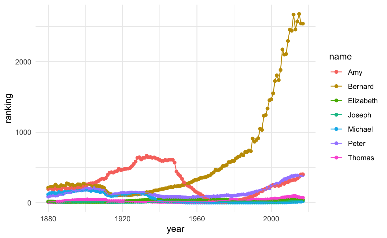
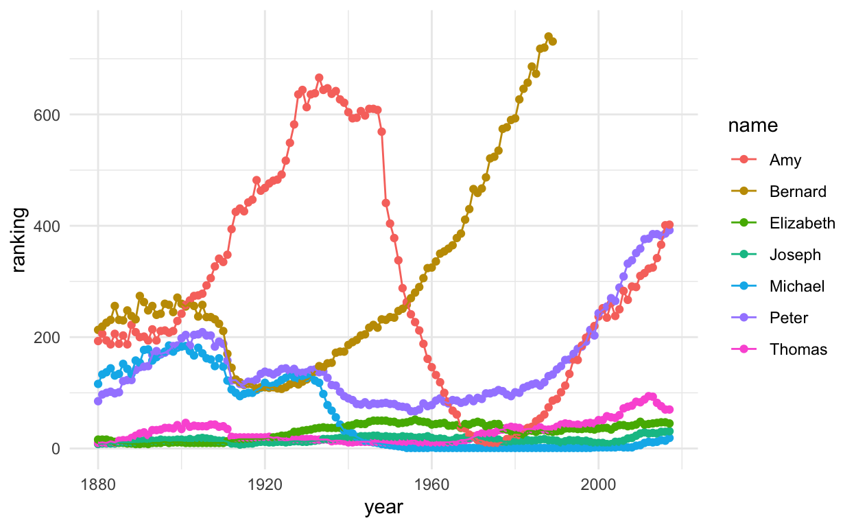
Many of these names are ranked pretty high fairly consistently.
allRanked %>%
  filter(name %in% candidates[candidate_status]) %>%
  ggplot(., aes(year, ranking, col = name, group = name)) +
  geom_point() +
  geom_line() +
  theme_minimal()
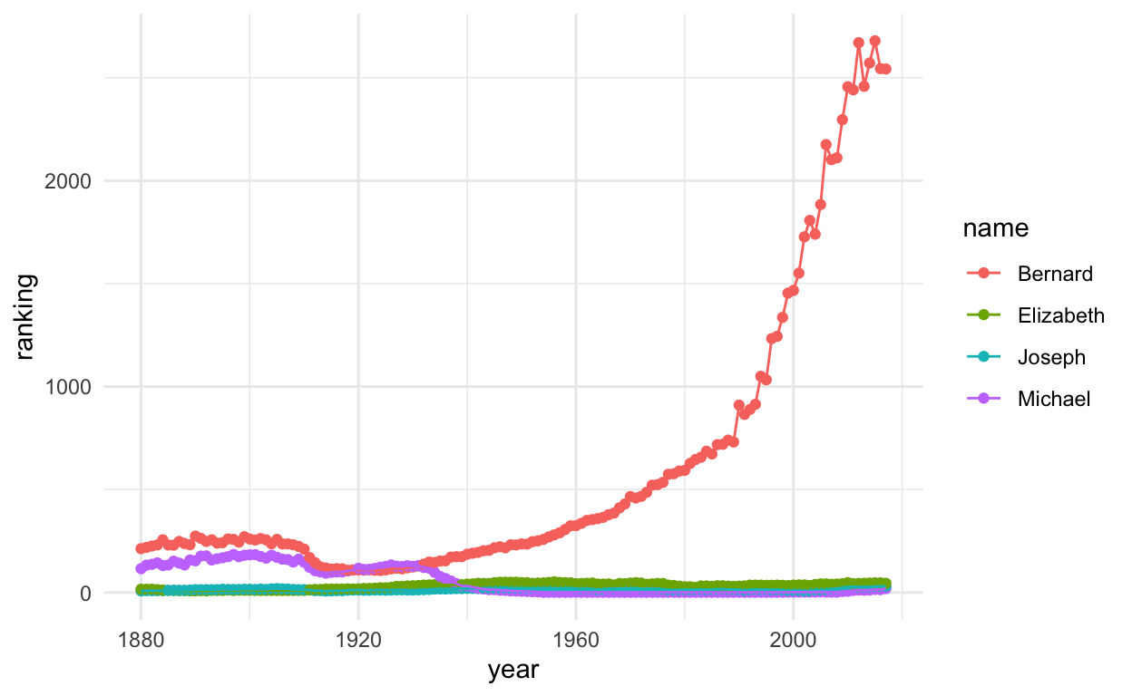
Alas, poor Bernard, let’s zoom in a bit.
allRanked %>%
  filter(name %in% candidates) %>%
  ggplot(., aes(year, ranking, col = name, group = name)) +
  geom_point() +
  geom_line() +
  theme_minimal() +
  ylim(c(0, 750))
It appears that these names often make the top 200 of baby names each year.
What are the average and best ranks across time?
allRanked %>%
  filter(name %in% candidates) %>%
  group_by(name) %>%
  summarise(avgRank = mean(ranking), bestRank = min(ranking)) %>%
  arrange(avgRank)
# A tibble: 7 x 3
  name      avgRank bestRank
  <chr>       <dbl>    <int>
1 Joseph       15.9        7
2 Thomas       30.4       10
3 Elizabeth    30.9        8
4 Michael      60.3        1
5 Peter       152.        67
6 Amy         288.         9
7 Bernard     594.       107
Joseph has the best average rank, but only Michael reached the top spot at one point in history.
How consistently were these names in the top 200, 100, or 50 spot over time?
allRanked %>%
  filter(ranking <= 200) %>%
  group_by(name) %>%
  summarise(count = n()) %>%
  arrange(desc(count)) %>%
  filter(name %in% candidates)
# A tibble: 7 x 2
  name      count
  <chr>     <int>
1 Elizabeth   138
2 Joseph      138
3 Michael     138
4 Thomas      138
5 Peter       112
6 Amy          48
7 Bernard      32
allRanked %>%
filter(ranking <= 100) %>%
group_by(name) %>%
summarise(count = n()) %>%
arrange(desc(count)) %>%
filter(name %in% candidates)
# A tibble: 6 x 2
  name      count
  <chr>     <int>
1 Elizabeth   138
2 Joseph      138
3 Thomas      138
4 Michael      89
5 Peter        43
6 Amy          28
allRanked %>%
filter(ranking <= 50) %>%
group_by(name) %>%
summarise(count = n()) %>%
arrange(desc(count)) %>%
filter(name %in% candidates)
# A tibble: 5 x 2
  name      count
  <chr>     <int>
1 Joseph      138
2 Elizabeth   137
3 Thomas      120
4 Michael      80
5 Amy          19
Out of 138 years of data, Joseph has always been in the top 50 of baby names. Elizabeth misses perfection by one year. Peter doesn’t crack the top 50 ceiling, but makes it into the top 100. Bernard manages to be in the top 200 for 32 years. It seems like these candidates are taking “name recognition” benefits a bit too far.
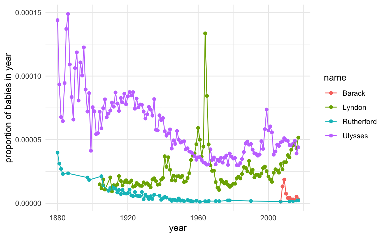
What does this mean for the presidential hopefuls? We love a good George, John, or James for president, but we’ve also had a Millard and Rutherford, so it’s anyone’s guess.
presidents <- c("George", "John", "Thomas", "James", "Andrew", "Martin", "William", "Zachary", "Millard", "Franklin", "Abraham", "Ulysses", "Rutherford", "Chester", "Grover", "Benjamin", "Theodore", "Woodrow", "Warren", "Calvin", "Herbert", "Harry", "Dwight", "Lyndon", "Richard", "Gerald", "Ronald", "Barack", "Donald")
presidentData <- babynames %>%
filter(name %in% presidents) %>%
group_by(year, name) %>%
summarise(count = sum(n))
presidentData <- merge(presidentData, yearTotals, by.x = "year", by.y = "year")
presidentData$prop <- presidentData$count / presidentData$yearTotal
presidentPop <- presidentData %>%
group_by(name) %>%
summarise(averageProp = mean(prop)) %>%
arrange(desc(averageProp))
presidentPop$id <- 1:nrow(presidentPop)
presidentData <- merge(presidentData, presidentPop, by.x = "name", by.y = "name")
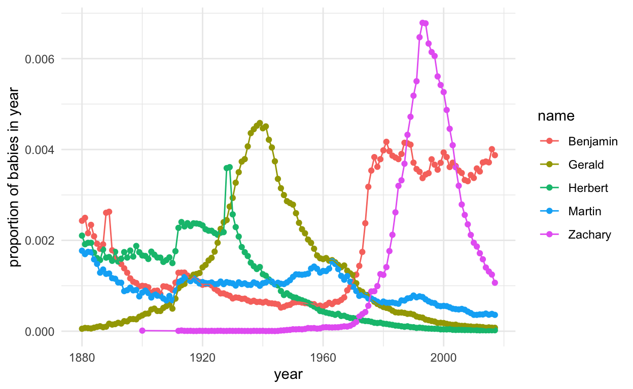
ggplot(subset(presidentData, id %in% 1:5), aes(year, prop, col = name, group = name)) +
geom_point() +
geom_line() +
theme_minimal() +
ylab("proportion of babies in year")
ggplot(subset(presidentData, id %in% 6:10), aes(year, prop, col = name, group = name)) +
  geom_point() +
  geom_line() +
  theme_minimal() +
  ylab("proportion of babies in year")
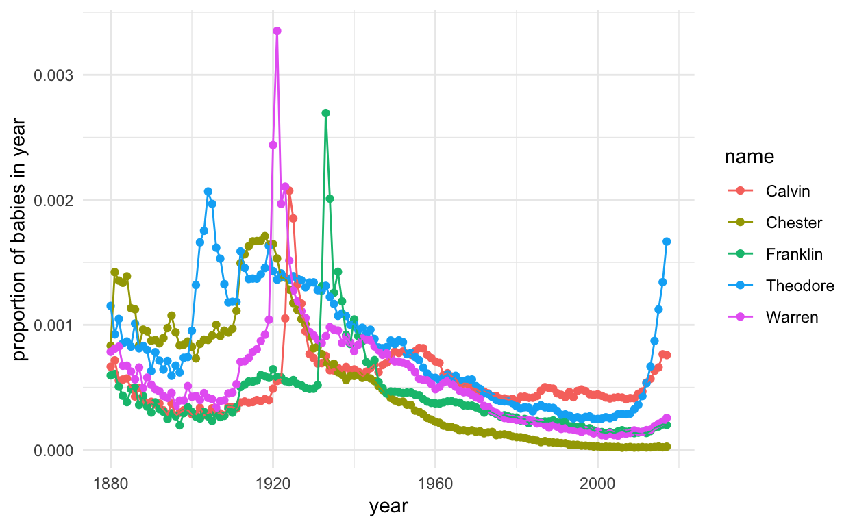
ggplot(subset(presidentData, id %in% 11:15), aes(year, prop, col = name, group = name)) +
  geom_point() +
  geom_line() +
  theme_minimal() +
  ylab("proportion of babies in year")
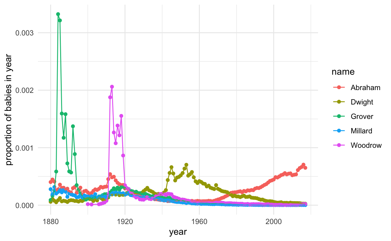
ggplot(subset(presidentData, id %in% 16:20), aes(year, prop, col = name, group = name)) +
  geom_point() +
  geom_line() +
  theme_minimal() +
  ylab("proportion of babies in year")
ggplot(subset(presidentData, id %in% 21:25), aes(year, prop, col = name, group = name)) +
  geom_point() +
  geom_line() +
  theme_minimal() +
  ylab("proportion of babies in year")
ggplot(subset(presidentData, id %in% 26:30), aes(year, prop, col = name, group = name)) +
  geom_point() +
  geom_line() +
  theme_minimal() +
  ylab("proportion of babies in year")