This is super tardy for Thanksgiving, but since Christmas is around the corner, and often there is a similar food vibe, here we go anyway…
Who travels most?
Trying to break down by community type, age, and gender, leaves bins too sparse.
look <- tg %>%
  filter(celebrate == "Yes") %>%
  group_by(travel, community_type, age, gender) %>%
  summarise(count = n())

summary(look$count) ## too sparse
   Min. 1st Qu.  Median    Mean 3rd Qu.    Max.
  1.000   4.500   8.000   9.899  13.000  38.000
Let’s first just look at travel by community type.
travelCommunity <- tg %>%
  filter(celebrate == "Yes") %>%
  group_by(travel, community_type) %>%
  summarise(count = n()) %>%
  filter(!is.na(community_type) & !is.na(travel)) %>%
  left_join(., tg %>% filter(celebrate == "Yes") %>% group_by(community_type) %>% summarise(total = n())) %>%
  mutate(percent = count / total)

ggplot(data = travelCommunity, aes(x = travel, y = percent, fill = community_type)) +
  geom_bar(stat = "identity", position = position_dodge()) +
  coord_flip()
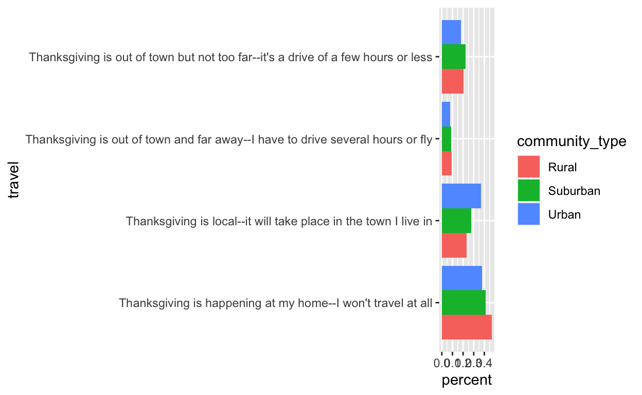
Ah, labels are a mess! Luckily, there is a natural breakpoint (—).
travelCommunity$travel2 <- unlist(lapply(strsplit(as.character(travelCommunity$travel), "--"), function(x) {
  paste(x[1], "\n", x[2], collapse = "")
}))

ggplot(data = travelCommunity, aes(x = travel2, y = percent, fill = community_type)) +
  geom_bar(stat = "identity", position = position_dodge()) +
  coord_flip() +
  xlab("")
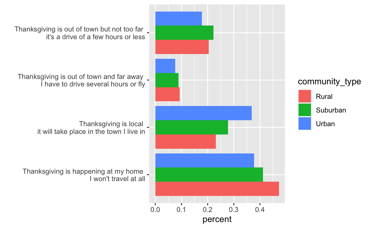
Having to specify the xlab as empty instead of the ylab that it ends up with due to the coord_flip was unexpected.
Now let’s look at travel by age.
travelAge <- tg %>%
  filter(celebrate == "Yes") %>%
  group_by(travel, age) %>%
  summarise(count = n()) %>%
  filter(!is.na(age) & !is.na(travel)) %>%
  left_join(., tg %>% filter(celebrate == "Yes") %>% group_by(age) %>% summarise(total = n())) %>%
  mutate(percent = count / total)

travelAge$travel2 <- unlist(lapply(strsplit(as.character(travelAge$travel), "--"), function(x) {
  paste(x[1], "\n", x[2], collapse = "")
})) ## similarly break up label
Here we need to reverse the order of age because of the coord_flip.
ggplot(data = travelAge, aes(x = travel2, y = percent, fill = age)) +
  geom_bar(stat = "identity", position = position_dodge()) +
  coord_flip() ## need to reverse order of age
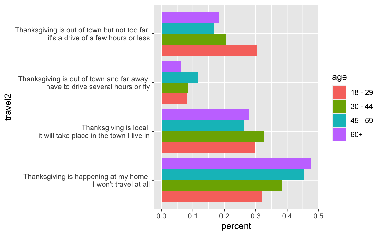
All the things that don’t work.
ggplot(data = travelAge, aes(x = travel2, y = percent, fill = age)) +
  geom_bar(stat = "identity", position = position_dodge()) +
  coord_flip() +
  scale_x_discrete(limits = rev(levels(travelAge$age))) ## nope

ggplot(data = travelAge, aes(x = travel2, y = percent, fill = age)) +
  geom_bar(stat = "identity", position = position_dodge()) +
  coord_flip() +
  scale_y_discrete(limits = rev(levels(travelAge$age))) ## nope

## set limits before flipping?
ggplot(data = travelAge, aes(x = travel2, y = percent, fill = age)) +
  geom_bar(stat = "identity", position = position_dodge()) +
  scale_y_discrete(limits = rev(levels(travelAge$age))) +
  coord_flip() ## nope

ggplot(data = travelAge, aes(x = travel2, y = percent, fill = age)) +
  geom_bar(stat = "identity", position = position_dodge()) +
  scale_x_discrete(limits = rev(levels(travelAge$age))) +
  coord_flip() ## nope
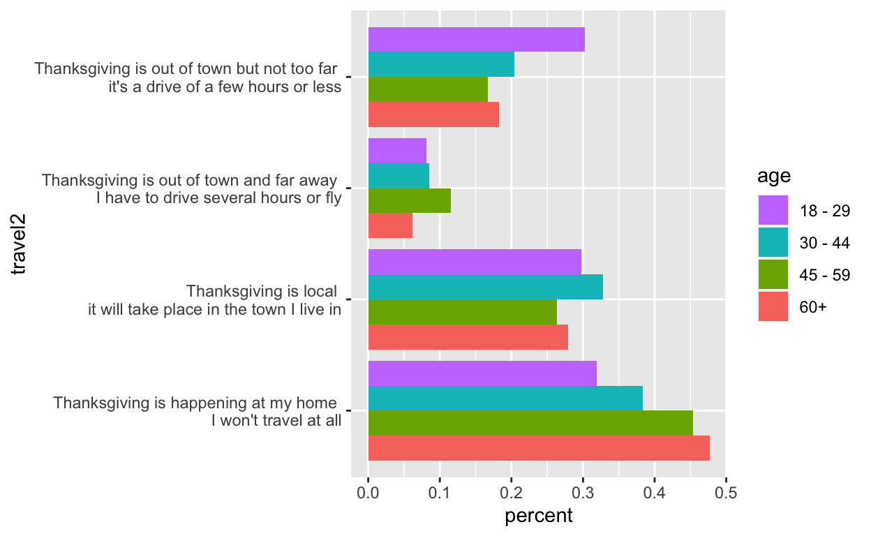
Finally, the winner!

ggplot(data = travelAge %>% mutate(age = fct_rev(age)), aes(x = travel2, y = percent, fill = age)) +
  geom_bar(stat = "identity", position = position_dodge()) +
  coord_flip() +
  scale_fill_discrete(guide = guide_legend(reverse = TRUE))
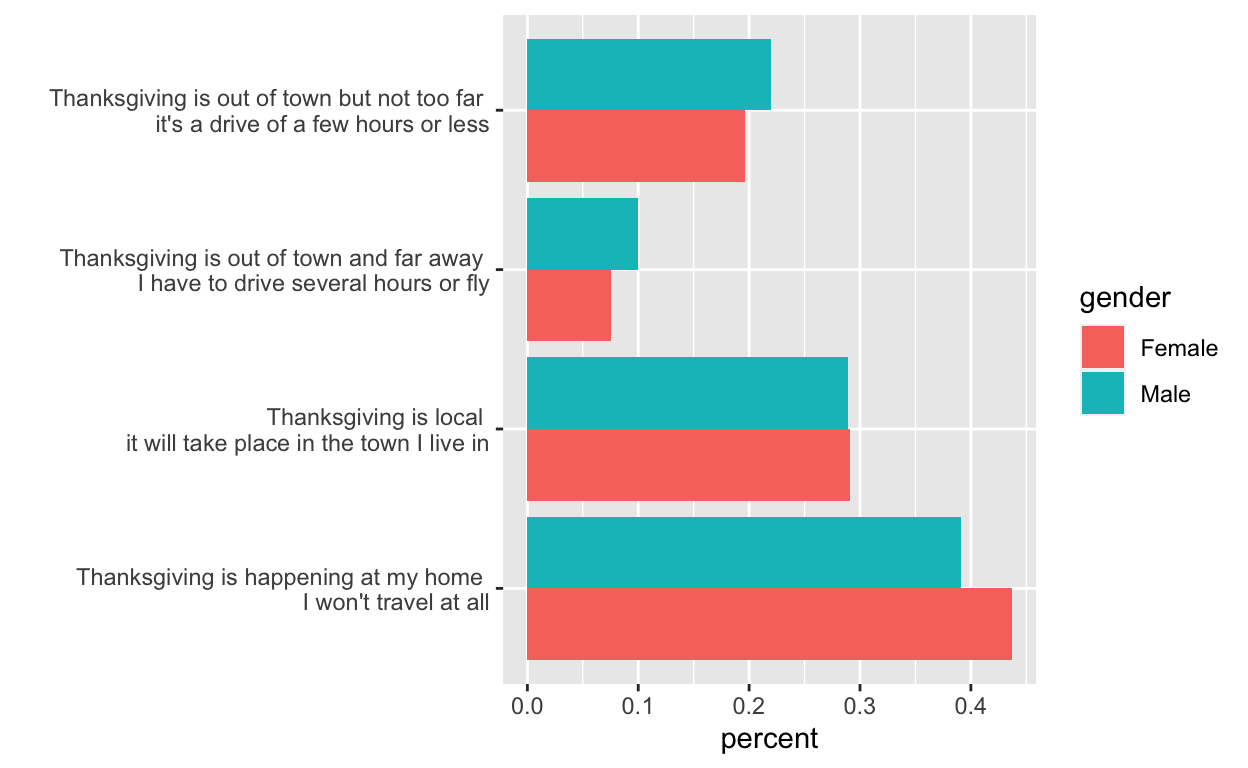
How about travel by gender?
travelGender <- tg %>%
  filter(celebrate == "Yes") %>%
  group_by(travel, gender) %>%
  summarise(count = n()) %>%
  filter(!is.na(gender) & !is.na(travel)) %>%
  left_join(., tg %>% filter(celebrate == "Yes") %>% group_by(gender) %>% summarise(total = n())) %>%
  mutate(percent = count / total)

travelGender$travel2 <- unlist(lapply(strsplit(as.character(travelGender$travel), "--"), function(x) {
  paste(x[1], "\n", x[2], collapse = "")
})) ## similarly break up label

ggplot(data = travelGender, aes(x = travel2, y = percent, fill = gender)) +
  geom_bar(stat = "identity", position = position_dodge()) +
  coord_flip() +
  xlab("")
Who is shopping and who is working on Black Friday?
There is a small sample size here, so I’m just going to report some simple summary tables.
income <- tg %>%
  filter(celebrate == "Yes") %>%
  group_by(family_income) %>%
  summarise(work = length(which(work_retail == "Yes")), shop = length(which(black_friday == "Yes"))) %>%
  left_join(., tg %>% filter(celebrate == "Yes") %>% group_by(family_income) %>% summarise(total = n())) %>%
  mutate(propW = work / total, propS = shop / total) %>%
  filter(!is.na(family_income))
# A tibble: 3 x 2
  work_black_friday count
* <fct>             <int>
1 Doesn't apply         7
2 No                   20
3 Yes                  43
## small sample size, can't do much
tg %>%
filter(work_retail == "Yes") %>%
group_by(gender) %>%
summarise(count = n())
# A tibble: 3 x 2
  gender count
* <fct>  <int>
1 Female    31
2 Male      38
3 <NA> 1# A tibble: 5 x 2
age count
* <fct> <int>
1 18 - 29 26
2 30 - 44 21
3 45 - 59 15
4 60+ 7
5 <NA> 1# A tibble: 3 x 2
work_black_friday count
* <fct> <int>
1 Doesn't apply 7
2 No 20
3 Yes 43I want to reorder based on money not alphabetical order.
levels(income$family_income) ## want to reorder
 [1] "$0 to $9,999"         "$10,000 to $24,999"
 [3] "$100,000 to $124,999" "$125,000 to $149,999"
 [5] "$150,000 to $174,999" "$175,000 to $199,999"
 [7] "$200,000 and up"      "$25,000 to $49,999"
 [9] "$50,000 to $74,999"   "$75,000 to $99,999"
[11] "Prefer not to answer"
intstep <- levels(income$family_income)[order(nchar(levels(income$family_income)))]
intstep ## by number of characters, works except for and up
 [1] "$0 to $9,999"         "$200,000 and up"
 [3] "$10,000 to $24,999"   "$25,000 to $49,999"
 [5] "$50,000 to $74,999"   "$75,000 to $99,999"
 [7] "$100,000 to $124,999" "$125,000 to $149,999"
 [9] "$150,000 to $174,999" "$175,000 to $199,999"
[11] "Prefer not to answer"
test <- fct_relevel(income$family_income, c(intstep[1], intstep[3:10], intstep[2], intstep[11]))
levels(test)
 [1] "$0 to $9,999"         "$10,000 to $24,999"
 [3] "$25,000 to $49,999"   "$50,000 to $74,999"
 [5] "$75,000 to $99,999"   "$100,000 to $124,999"
 [7] "$125,000 to $149,999" "$150,000 to $174,999"
 [9] "$175,000 to $199,999" "$200,000 and up"
[11] "Prefer not to answer"income$family_income <- fct_relevel(income$family_income, c(intstep[1], intstep[3:10], intstep[2], intstep[11]))
levels(test)
 [1] "$0 to $9,999"         "$10,000 to $24,999"
 [3] "$25,000 to $49,999"   "$50,000 to $74,999"
 [5] "$75,000 to $99,999"   "$100,000 to $124,999"
 [7] "$125,000 to $149,999" "$150,000 to $174,999"
 [9] "$175,000 to $199,999" "$200,000 and up"
[11] "Prefer not to answer"byIncome$family_income <- fct_relevel(byIncome$family_income, c(intstep[1], intstep[3:10], intstep[2], intstep[11]))
byIncome
# A tibble: 12 x 2
   family_income        count
   <fct>                <int>
 1 $0 to $9,999            10
 2 $10,000 to $24,999       8
 3 $100,000 to $124,999     4
 4 $125,000 to $149,999     1
 5 $150,000 to $174,999     2
 6 $175,000 to $199,999     1
 7 $200,000 and up          5
 8 $25,000 to $49,999      17
 9 $50,000 to $74,999       5
10 $75,000 to $99,999       9
11 Prefer not to answer     7
12 <NA>                     1
Pie!
The question asks “Which type of pie is typically served at your Thanksgiving dinner? Please select all that apply.” Each column represents a type of pie.
   pie1 pie2   pie3      pie4 pie5 pie6  pie7  pie8    pie9
1 Apple <NA>   <NA>      <NA> <NA> <NA>  <NA>  <NA>    <NA>
2 Apple <NA>   <NA> Chocolate <NA> <NA>  <NA>  <NA> Pumpkin
3 Apple <NA> Cherry      <NA> <NA> <NA> Peach Pecan Pumpkin
4  <NA> <NA>   <NA>      <NA> <NA> <NA>  <NA> Pecan Pumpkin
5 Apple <NA>   <NA>      <NA> <NA> <NA>  <NA>  <NA> Pumpkin
6  <NA> <NA>   <NA>      <NA> <NA> <NA>  <NA>  <NA>    <NA>
         pie10 pie11                  pie12                 pie13
1         <NA>  <NA>                   <NA>                  <NA>
2         <NA>  <NA> Other (please specify) Derby, Japanese fruit
3 Sweet Potato  <NA>                   <NA>                  <NA>
4         <NA>  <NA>                   <NA>                  <NA>
5         <NA>  <NA>                   <NA>                  <NA>
6 Sweet Potato <NA> Other (please specify) Blueberry piecbind.data.frame(
type = (tg %>% select(contains("pie")) %>% apply(., 2, function(x) {
x[which(!is.na(x))[1]]
})),
count = (tg %>% select(contains("pie")) %>% apply(., 2, function(x) {
length(which(!is.na(x)))
}))
) %>% arrange(desc(count))
                        type count
pie9                 Pumpkin   729
pie1                   Apple   514
pie8                   Pecan   342
pie10           Sweet Potato   152
pie4               Chocolate   133
pie3                  Cherry   113
pie12 Other (please specify)    71
pie13  Derby, Japanese fruit    71
pie11                   None    40
pie6                Key lime    39
pie5           Coconut cream    36
pie2              Buttermilk    35
pie7                   Peach    34
Since “Other (please specify)” has the same count as “Derby, Japanese fruit”, I’m going to assume this type of pie is where they specified. This will impact the count of pies per household.
tg %>%
  select(contains("pie")) %>%
  mutate(numPies = apply(., 1, function(x) {
    length(which(!is.na(x)))
  })) %>%
  mutate(isOther = apply(., 1, function(x) {
    as.numeric(!is.na(x[12]))
  })) %>%
  mutate(numPiesAdj = numPies - isOther) %>%
  ggplot(., aes(numPiesAdj)) +
  geom_histogram(binwidth = 1, col = "black", fill = "white")
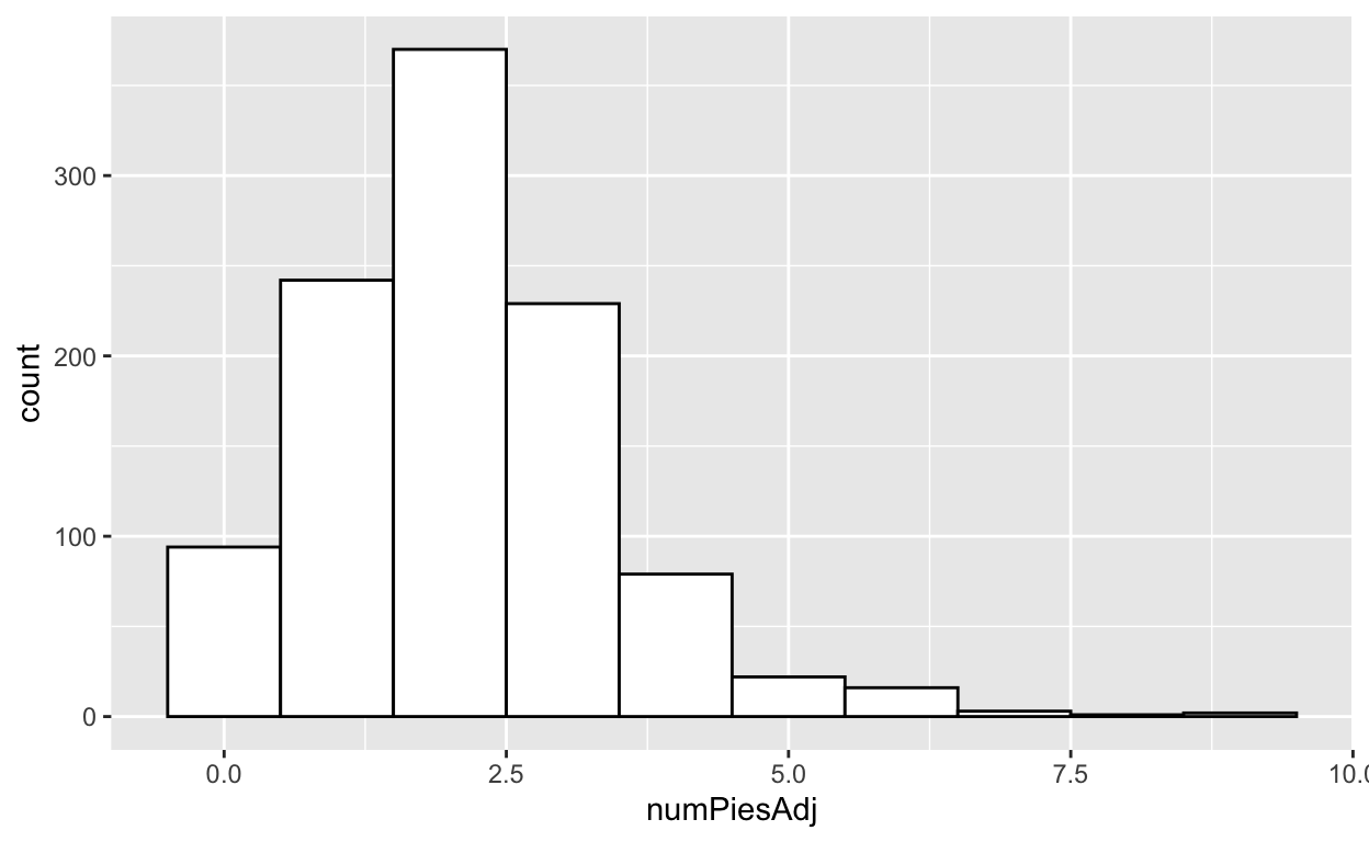
Please invite me to the households that serve over five different types of pie per holiday (but perhaps people rotate among types of pies each year and don’t actually have them all at one time).
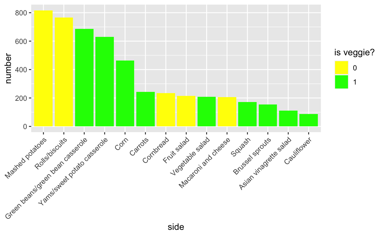
Veggies

Sides are reported similarly to pie. How do veggies fare in the side dish line up?
sideNum <- tg %>%
  select(contains("side")) %>%
  apply(., 2, function(x) {
    length(which(!is.na(x)))
  }) %>%
  as.data.frame() %>%
  t() %>%
  as.data.frame()

sideNames <- tg %>%
  select(contains("side")) %>%
  apply(., 2, function(x) {
    x[which(!is.na(x))[1]]
  }) %>%
  as.data.frame()

names(sideNum) <- sideNames[, 1]

sideNames[, 1]
 [1] Brussel sprouts                  Carrots
 [3] Cauliflower                      Corn
 [5] Cornbread                        Fruit salad
 [7] Green beans/green bean casserole Macaroni and cheese
 [9] Mashed potatoes                  Rolls/biscuits
[11] Squash                           Vegetable salad
[13] Yams/sweet potato casserole      Other (please specify)
[15] Asian vinagrette salad
15 Levels: Asian vinagrette salad Brussel sprouts ... Yams/sweet potato casseroleggplot(data = sideNum, aes(x = reorder(side, -num), y = num, fill = as.factor(isVeggie))) +
geom_bar(stat = "identity", position = position_dodge()) +
theme(axis.text.x = element_text(angle = 45, hjust = 1)) +
ylab("number") +
xlab("side") +
scale_fill_manual(values = c("yellow", "green"), name = "is veggie?")
# https://stackoverflow.com/questions/25664007/reorder-bars-in-geom-bar-ggplot2
Who can compete with potatoes and carbs?
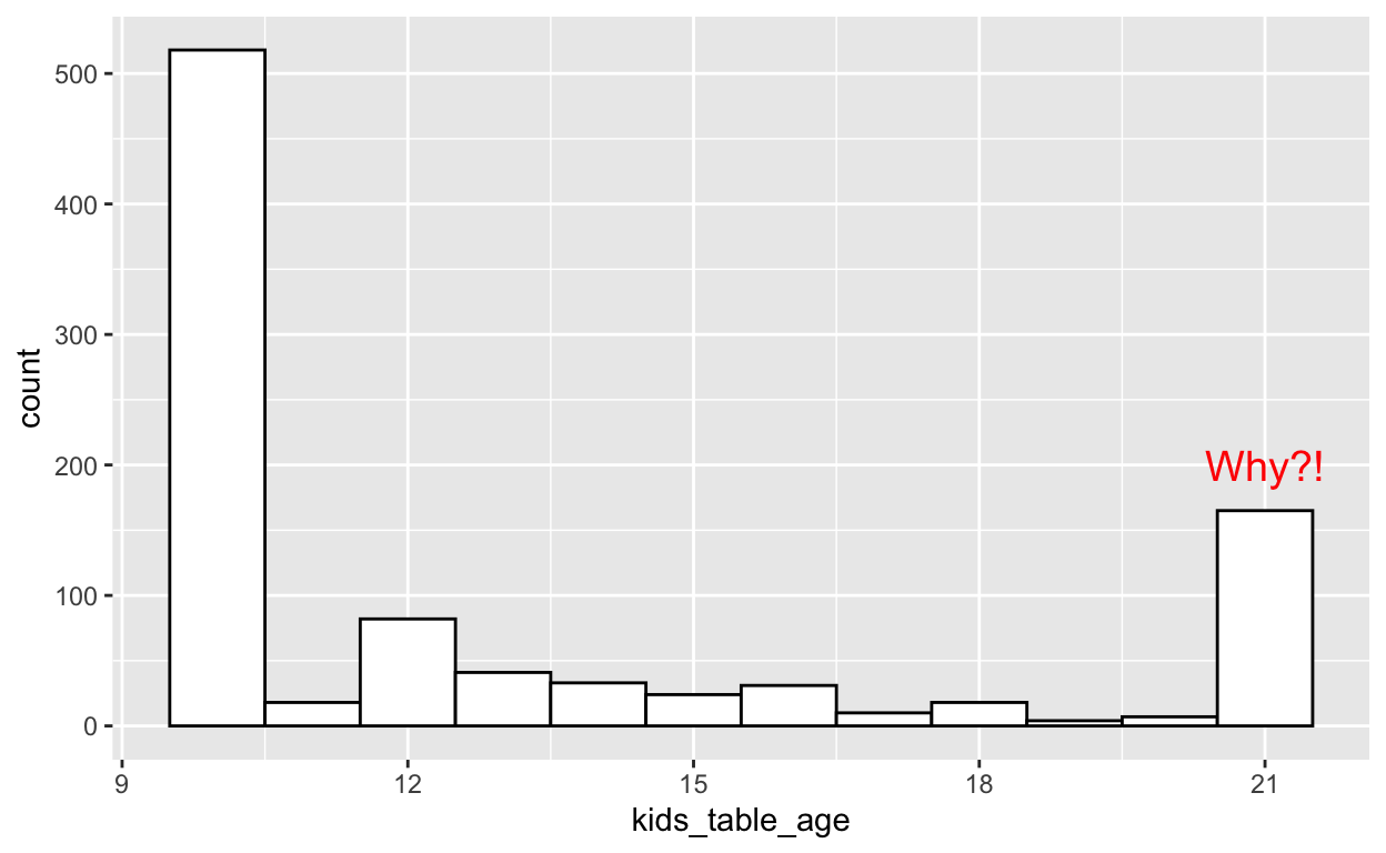
And the most controversial topic: the kids’ table
Yes, I’m a little salty for being at the kids’ table too many times.

Here the question answered was “What’s the age cutoff at your”kids’ table" at Thanksgiving?". It appears that there is a non-neglible number of people who have a 21+ rule for the kids’ table.
levels(tg$kids_table_age)
 [1] "10 or younger" "11"            "12"            "13"
 [5] "14"            "15"            "16"            "17"
[9] "18" "19" "20" "21 or older" tg$kids_table_age <- as.numeric(str_replace_all(as.character(tg$kids_table_age), "or .*", ""))
ggplot(tg, aes(kids_table_age)) +
geom_histogram(binwidth = 1, col = "black", fill = "white") +
annotate("text", x = 21, y = 200, label = "Why?!", col = "red", size = 5)
Happy Holidays!