It has been a LONG time since I last participated in Tidy Tuesday. Apologies #rstats world! It turns out getting a PhD is… alot. But I obviously had to return for the Squirrel Census.
library(dplyr)
library(stringr)
library(kableExtra)
library(ggplot2)
library(purrr)
library(magrittr)

setwd("~/Desktop/tidytuesday/data/2019/2019-10-29")

sq <- read.csv("nyc_squirrels.csv", stringsAsFactors = F)
names(sq)
 [1] "long"
 [2] "lat"
 [3] "unique_squirrel_id"
 [4] "hectare"
 [5] "shift"
 [6] "date"
 [7] "hectare_squirrel_number"
 [8] "age"
 [9] "primary_fur_color"
[10] "highlight_fur_color"
[11] "combination_of_primary_and_highlight_color"
[12] "color_notes"
[13] "location"
[14] "above_ground_sighter_measurement"
[15] "specific_location"
[16] "running"
[17] "chasing"
[18] "climbing"
[19] "eating"
[20] "foraging"
[21] "other_activities"
[22] "kuks"
[23] "quaas"
[24] "moans"
[25] "tail_flags"
[26] "tail_twitches"
[27] "approaches"
[28] "indifferent"
[29] "runs_from"
[30] "other_interactions"
[31] "lat_long"
[32] "zip_codes"
[33] "community_districts"
[34] "borough_boundaries"
[35] "city_council_districts"
[36] "police_precincts"
What weird stuff can we find? The highlight_fur_color field catches my eye. Who knew squirrels were into highlights?
tt <- sq %>%
  group_by(unique_squirrel_id) %>%
  summarise(primary_fur_color = primary_fur_color[1]) %>%
  group_by(primary_fur_color) %>%
  summarise(count = n()) %>%
  arrange(desc(count)) %>%
  as.data.frame()

kable(tt) %>% kable_styling()
| primary_fur_color | count |
|---|---|
| Gray | 2468 |
| Cinnamon | 392 |
| Black | 103 |
| NA | 55 |
tt <- sq %>%
  group_by(unique_squirrel_id) %>%
  summarise(primary_fur_color = primary_fur_color[1], highlight_fur_color = highlight_fur_color[1]) %>%
  group_by(primary_fur_color, highlight_fur_color) %>%
  summarise(count = n()) %>%
  arrange(desc(count)) %>%
  as.data.frame()

kable(tt) %>% kable_styling()
| primary_fur_color | highlight_fur_color | count |
|---|---|---|
| Gray | NA | 894 |
| Gray | Cinnamon | 750 |
| Gray | White | 487 |
| Gray | Cinnamon, White | 265 |
| Cinnamon | Gray | 162 |
| Cinnamon | White | 94 |
| Black | NA | 74 |
| Cinnamon | NA | 62 |
| Cinnamon | Gray, White | 58 |
| NA | NA | 55 |
| Gray | Black, Cinnamon, White | 32 |
| Gray | Black | 24 |
| Black | Cinnamon | 15 |
| Cinnamon | Black | 10 |
| Gray | Black, Cinnamon | 9 |
| Black | Gray | 8 |
| Gray | Black, White | 7 |
| Black | Cinnamon, White | 3 |
| Cinnamon | Black, White | 3 |
| Cinnamon | Gray, Black | 3 |
| Black | White | 2 |
| Black | Gray, White | 1 |
I’m kind of surprised that gray with black highlights is so uncommon. But to be fair, that surprise is based on absolutely no knowlege of NYC squirrels. Enlighten me!
The next weird thing I wanted to dig in was the other_activities field. Look at some of these gems.
unique(sq$other_activities)[3:12]
 [1] "wrestling with mother"
 [2] "grooming"
 [3] "walking"
 [4] "moving slowly"
 [5] "sitting"
 [6] "eating (ate upside down on a tree — #jealous)"
 [7] "running (with nut)"
 [8] "playing with #5"
 [9] "hiding nut"
[10] "drank from a pond of rain water"
I’m interested in the squirrel interactions.
interactions <- sq[str_which(sq$other_activities, "#"), ]

# interactions[1, ]

interactions <- interactions[-1, ] ## get rid of #jealous
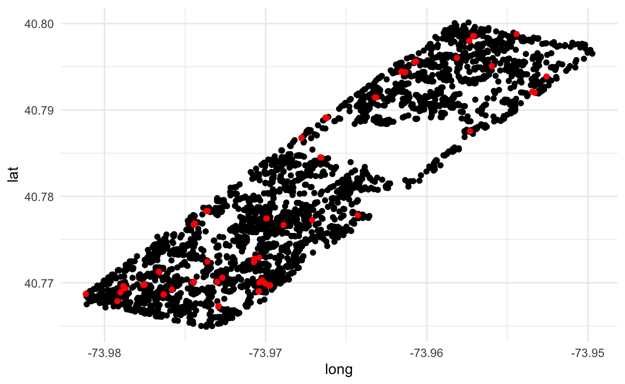
The first thing I want to know is whether this level of detail is concentrated in one pocket (due to a few really intense data collectors). Actually, no!
ggplot(sq, aes(long, lat)) +
  geom_point() +
  geom_point(data = interactions, aes(long, lat), col = "red") +
  theme_minimal()
For each interaction, who is the other squirrel?
nums <- unlist(map(str_split(interactions$other_activities, "#"), 2)) ## grab the number
justNums <- str_replace_all(nums, "[^0-9]", "") ## get rid of the extra junk
interactions$otherSquirrel <- justNums
Ok, now for some data munging. If we look at the unique_squirrel_id field, it isn’t a perfect paste of “Hectare ID” + “Shift” + “Date” + “Hectare Squirrel Number.” The hectare ID has to be un-padded, the date has to be striped of the year, and the squirrel number has to be padded. Here we go!
getBuddy <- function(x) {
  unpadHectare <- str_sub(interactions$hectare[x], str_locate(interactions$hectare[x], "[^0]")[1], str_length(interactions$hectare[x]))
  # https://stat.ethz.ch/pipermail/r-help/2010-October/255450.html
  newDate <- str_sub(interactions$date[x], 1, 4)
  paddedSquirrel <- str_pad(interactions$otherSquirrel[x], width = 2, side = "left", pad = "0")
  id <- paste(unpadHectare, interactions$shift[x], newDate, paddedSquirrel, sep = "-")
  subset(sq, unique_squirrel_id == id)
}
Pause for some fun.
interactions$other_activities[31]
[1] "canoodling w/ #9"Back to business.
buddies <- map(1:nrow(interactions), getBuddy)

map(buddies, nrow) %>%
  unlist() %>%
  summary() ## check that everyone got a buddy
   Min. 1st Qu.  Median    Mean 3rd Qu.    Max.
1 1 1 1 1 1 It looks like squirrels interact with squirrels like them in terms of age and coloring. But of course there is a big disparity in age and color overall, so I don’t want to read too much into this.
tt <- interactions %>%
  group_by(age, otherSquirrelAge) %>%
  summarise(count = n())

kable(tt) %>% kable_styling()
| age | otherSquirrelAge | count |
|---|---|---|
| Adult | Adult | 52 |
| Adult | Juvenile | 6 |
| Juvenile | Adult | 2 |
| Juvenile | Juvenile | 5 |
| NA | NA | 6 |
tt <- interactions %>%
  group_by(primary_fur_color, otherSquirrelPrimaryFurColor) %>%
  summarise(count = n()) %>%
  arrange(desc(count))

kable(tt) %>% kable_styling()
| primary_fur_color | otherSquirrelPrimaryFurColor | count |
|---|---|---|
| Gray | Gray | 51 |
| Cinnamon | Gray | 6 |
| Gray | Cinnamon | 6 |
| Cinnamon | Cinnamon | 4 |
| Gray | NA | 2 |
| Black | Gray | 1 |
| Gray | Black | 1 |
tt <- interactions %>%
  group_by(primary_fur_color, highlight_fur_color, otherSquirrelPrimaryFurColor, otherSquirrelHighlightFurColor) %>%
  summarise(count = n()) %>%
  arrange(desc(count))


kable(tt) %>% kable_styling()
| primary_fur_color | highlight_fur_color | otherSquirrelPrimaryFurColor | otherSquirrelHighlightFurColor | count |
|---|---|---|---|---|
| Gray | NA | Gray | NA | 20 |
| Gray | Cinnamon | Gray | Cinnamon | 11 |
| Gray | Cinnamon, White | Gray | Cinnamon, White | 4 |
| Gray | NA | Gray | Cinnamon | 4 |
| Cinnamon | Gray | Gray | Cinnamon | 2 |
| Cinnamon | Gray | Gray | NA | 2 |
| Cinnamon | Gray, White | Cinnamon | Gray, White | 2 |
| Cinnamon | White | Cinnamon | White | 2 |
| Gray | Cinnamon | Gray | White | 2 |
| Gray | Cinnamon | Gray | NA | 2 |
| Gray | White | Gray | Cinnamon | 2 |
| Gray | NA | Cinnamon | Gray | 2 |
| Black | NA | Gray | NA | 1 |
| Cinnamon | NA | Gray | Cinnamon, White | 1 |
| Cinnamon | NA | Gray | White | 1 |
| Gray | Cinnamon | Cinnamon | Gray | 1 |
| Gray | Cinnamon | NA | NA | 1 |
| Gray | Cinnamon, White | Cinnamon | NA | 1 |
| Gray | Cinnamon, White | Gray | White | 1 |
| Gray | Cinnamon, White | Gray | NA | 1 |
| Gray | White | Cinnamon | Gray | 1 |
| Gray | White | Cinnamon | NA | 1 |
| Gray | White | Gray | White | 1 |
| Gray | White | Gray | NA | 1 |
| Gray | NA | Black | NA | 1 |
| Gray | NA | Gray | Cinnamon, White | 1 |
| Gray | NA | Gray | White | 1 |
| Gray | NA | NA | NA | 1 |
So what have we learned? Not much, but there was some fun data wrangling + squirrels. Full disclosure, I did some not-tidy stuff in the exploratory phase, but in this post I took some extra time to switch back to the tidyverse. I admit, I had to refer back to this multiple times despite writing it.
Comments, suggestions, etc. are welcome –> @sastoudt