Week 15
setwd("~/Desktop/tidytuesday/data/2018/2018-07-10")
beers <- read_excel("week15_beers.xlsx", sheet = 1)
brewer <- read_excel("week15_beers.xlsx", sheet = 2)
beer <- inner_join(beers, brewer, by = c("brewery_id" = "id"))
byState <- beer %>%
  group_by(state) %>%
  summarise(numBrewer = length(unique(brewery_id)), count = n(), mabv = mean(abv, na.rm = T))
counties <- map_data("county")
state <- map_data("state")

stateInfo <- cbind.data.frame(abb = state.abb, name = tolower(state.name))

state <- inner_join(state, stateInfo, by = c("region" = "name"))

all_state <- inner_join(state, byState, by = c("abb" = "state"))
This palette isn’t very visually appealing, but in the spirit of beer, I’ll use it anyway.
# https://www.reddit.com/r/beer/comments/4gd24e/the_hex_colour_palette_of_beer/
beerPal <- c("#F3F993", "#F5F75C", "#F6F513", "#EAE615", "#E0D01B", "#D5BC26", "#CDAA37", "#C1963C", "#BE8C3A", "#BE823A", "#C17A37", "#BF7138", "#BC6733", "#B26033", "#A85839", "#985336", "#8D4C32", "#7C452D", "#6B3A1E", "#5D341A", "#4E2A0C", "#4A2727", "#361F1B", "#261716", "#231716", "#19100F", "#16100F", "#120D0C", "#100B0A", "#050B0A")
Where to Bar Crawl?
ggplot(data = state, mapping = aes(x = long, y = lat, group = group)) +
  geom_polygon(data = all_state, aes(fill = mabv), color = "grey") +
  labs(fill = "mabv") +
  scale_fill_gradientn(colors = beerPal) +
  theme_void() +
  geom_path(data = state, aes(x = long, y = lat, group = group), color = "black") +
  ggtitle("Where is the beer strongest?")
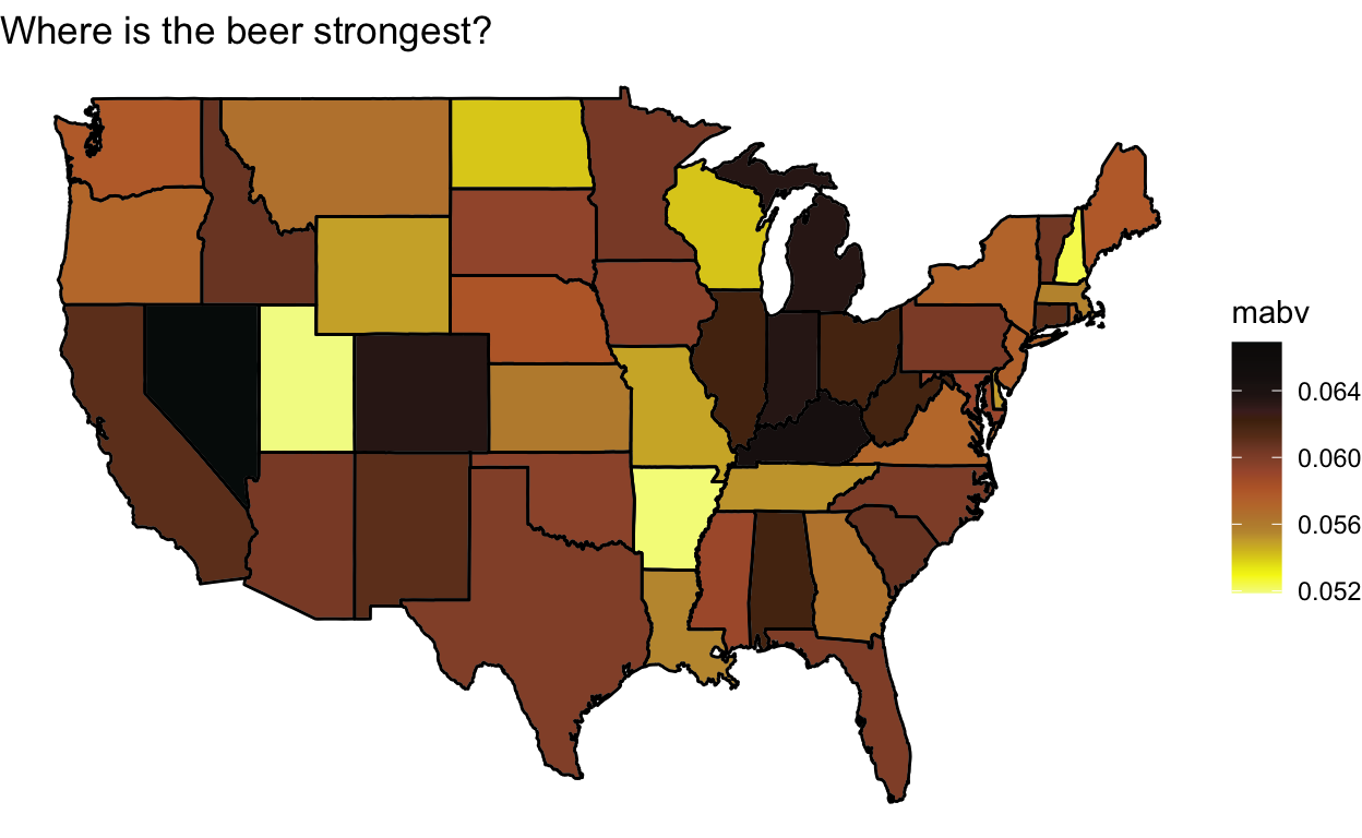
A stark (and believable) difference between Nevada and Utah.
ggplot(data = state, mapping = aes(x = long, y = lat, group = group)) +
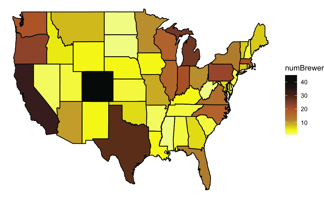
geom_polygon(data = all_state, aes(fill = numBrewer), color = "grey") +
labs(fill = "numBrewer") +
scale_fill_gradientn(colors = beerPal) +
theme_void() +
geom_path(data = state, aes(x = long, y = lat, group = group), color = "black") +
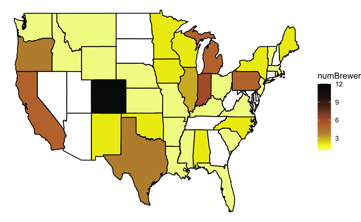
ggtitle("Where are the most breweries?")
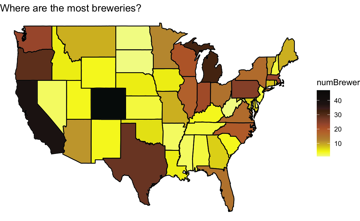
Colorado maintains it’s reputation.
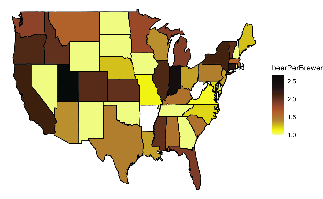
ggplot(data = state, mapping = aes(x = long, y = lat, group = group)) +
geom_polygon(data = all_state, aes(fill = count / numBrewer), color = "grey") +
labs(fill = "beerPerBrewer") +
scale_fill_gradientn(colors = beerPal) +
theme_void() +
geom_path(data = state, aes(x = long, y = lat, group = group), color = "black") +
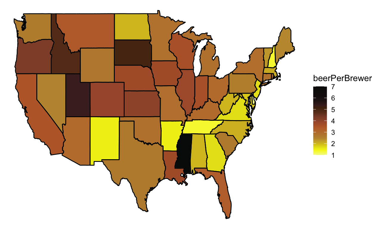
ggtitle("Where is the largest variety?")
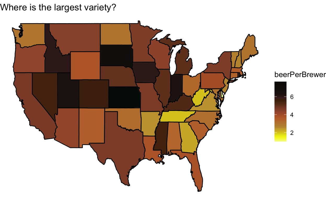
Surprisingly Kansas is where it is at!
beer %>%
  group_by(city, state) %>%
  summarise(count = n(), numBrewer = length(unique(brewery_id))) %>%
  arrange(desc(count))
# A tibble: 401 x 4
# Groups:   city [384]
   city         state count numBrewer
   <chr>        <chr> <int>     <int>
 1 Grand Rapids MI       66         3
 2 Chicago      IL       55         9
 3 Portland     OR       52        11
 4 Indianapolis IN       43         4
 5 San Diego    CA       42         8
 6 Boulder      CO       41         9
 7 Denver       CO       40         8
 8 Brooklyn     NY       38         4
 9 Seattle      WA       35         9
10 Longmont     CO       33         1
# … with 391 more rows
beer %>%
group_by(city, state) %>%
summarise(count = n(), numBrewer = length(unique(brewery_id))) %>%
arrange(desc(numBrewer))
# A tibble: 401 x 4
# Groups:   city [384]
   city          state count numBrewer
   <chr>         <chr> <int>     <int>
 1 Portland      OR       52        11
 2 Boulder       CO       41         9
 3 Chicago       IL       55         9
 4 Seattle       WA       35         9
 5 Austin        TX       25         8
 6 Denver        CO       40         8
 7 San Diego     CA       42         8
 8 Bend          OR       11         6
 9 Portland      ME       12         6
10 San Francisco CA       32         5
# … with 391 more rows
Somebody please tell me about the hidden gem of Grand Rapids. Apparently, it is Beer City, USA.
Styles
There are too many styles, so I pick some major ones and investigate them.
stout <- beer[str_detect(beer$style, "Stout"), ]
american <- beer[str_detect(beer$style, "American"), ]
ipa <- beer[str_detect(beer$style, "IPA"), ]
True American?
byStateA <- american %>%
group_by(state) %>%
summarise(numBrewer = length(unique(brewery_id)), count = n(), mabv = mean(abv, na.rm = T))
all_state <- inner_join(state, byStateA, by = c("abb" = "state"))
ggplot(data = state, mapping = aes(x = long, y = lat, group = group)) +
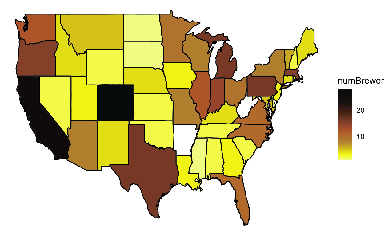
geom_polygon(data = all_state, aes(fill = numBrewer), color = "grey") +
labs(fill = "numBrewer") +
scale_fill_gradientn(colors = beerPal) +
theme_void() +
geom_path(data = state, aes(x = long, y = lat, group = group), color = "black")
ggplot(data = state, mapping = aes(x = long, y = lat, group = group)) +
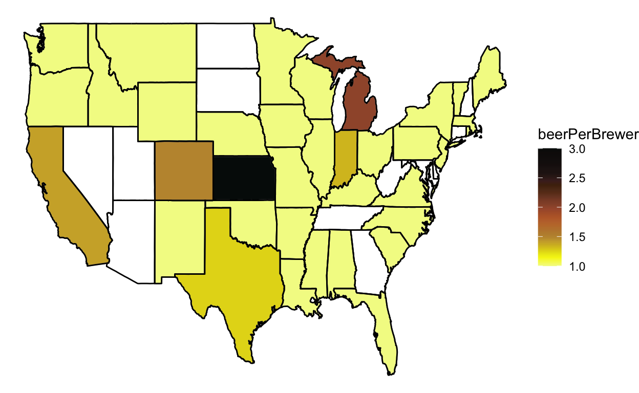
geom_polygon(data = all_state, aes(fill = count / numBrewer), color = "grey") +
labs(fill = "beerPerBrewer") +
scale_fill_gradientn(colors = beerPal) +
theme_void() +
geom_path(data = state, aes(x = long, y = lat, group = group), color = "black")
Mississippi: American Beer’s Hearland
Representing my namesake
byStateS <- stout %>%
  group_by(state) %>%
  summarise(numBrewer = length(unique(brewery_id)), count = n(), mabv = mean(abv, na.rm = T))

all_state <- inner_join(state, byStateS, by = c("abb" = "state"))

ggplot(data = state, mapping = aes(x = long, y = lat, group = group)) +
  geom_polygon(data = all_state, aes(fill = numBrewer), color = "grey") +
  labs(fill = "numBrewer") +
  scale_fill_gradientn(colors = beerPal) +
  theme_void() +
  geom_path(data = state, aes(x = long, y = lat, group = group), color = "black")
ggplot(data = state, mapping = aes(x = long, y = lat, group = group)) +
  geom_polygon(data = all_state, aes(fill = count / numBrewer), color = "grey") +
  labs(fill = "beerPerBrewer") +
  scale_fill_gradientn(colors = beerPal) +
  theme_void() +
  geom_path(data = state, aes(x = long, y = lat, group = group), color = "black")
What’s up with some states having no stouts?!
The controversial IPA
byStateI <- ipa %>%
  group_by(state) %>%
  summarise(numBrewer = length(unique(brewery_id)), count = n(), mabv = mean(abv, na.rm = T))

all_state <- inner_join(state, byStateI, by = c("abb" = "state"))

ggplot(data = state, mapping = aes(x = long, y = lat, group = group)) +
  geom_polygon(data = all_state, aes(fill = numBrewer), color = "grey") +
  labs(fill = "numBrewer") +
  scale_fill_gradientn(colors = beerPal) +
  theme_void() +
  geom_path(data = state, aes(x = long, y = lat, group = group), color = "black")
ggplot(data = state, mapping = aes(x = long, y = lat, group = group)) +
  geom_polygon(data = all_state, aes(fill = count / numBrewer), color = "grey") +
  labs(fill = "beerPerBrewer") +
  scale_fill_gradientn(colors = beerPal) +
  theme_void() +
  geom_path(data = state, aes(x = long, y = lat, group = group), color = "black")
## what's up with Utah?
ut <- beer[which(beer$state == "UT"), ]
ut[str_detect(ut$style, "IPA"), ] ## double counting
# A tibble: 8 x 12
  count.x   abv   ibu    id name.x style brewery_id ounces count.y
    <dbl> <dbl> <dbl> <dbl> <chr>  <chr>      <dbl>  <dbl>   <dbl>
1    1382 0.04     NA   644 Johnn… Amer…        399     16     400
2    2254 0.04     42  1925 Trade… Amer…        159     12     160
3    2255 0.073    83  1723 Hop N… Amer…        159     12     160
4    2258 0.073    82  1089 Hop N… Amer…        159     12     160
5    2300 0.09     75  1825 Squat… Amer…        302     12     303
6    2302 0.06     NA  1823 Wasat… Amer…        302     12     303
7    2303 0.06     NA  1682 Wasat… Amer…        302     12     303
8    2305 0.09     75  1680 Squat… Amer…        302     12     303
# … with 3 more variables: name.y <chr>, city <chr>, state <chr>
West Virginia and Arkansas are not into IPAs.
Variation in ABV
Which styles have the most variation in alcohol content (of the top 20 most prevalent styles) given their average value?
beer %>%
  group_by(style) %>%
  summarise(count = n(), coeffVarabv = mean(abv, na.rm = T) / sd(abv, na.rm = T)) %>%
  arrange(desc(count)) %>%
  head(20) %>%
  arrange(desc(coeffVarabv))
# A tibble: 20 x 3
   style                          count coeffVarabv
   <chr>                          <int>       <dbl>
 1 American Double / Imperial IPA   105       12.5
 2 Kölsch                           42       11.4
 3 American Amber / Red Lager        29       10.7
 4 American Blonde Ale              108       10.0
 5 Märzen / Oktoberfest             30        9.72
 6 Hefeweizen                        40        9.44
 7 American Pale Ale (APA)          245        8.63
 8 Cider                             37        7.58
 9 American Pale Wheat Ale           97        7.55
10 American IPA                     424        7.33
11 American Stout                    39        7.17
12 German Pilsener                   36        7.01
13 American Porter                   68        6.96
14 American Amber / Red Ale         133        6.62
15 American Pale Lager               39        6.27
16 American Brown Ale                70        5.97
17 American Black Ale                36        5.49
18 Fruit / Vegetable Beer            49        5.44
19 Saison / Farmhouse Ale            52        5.41
20 Witbier                           51        4.79
Fancy string matching for another time: match the beer style to the colors listed here.