Comic Book Characters

Data: Comic book characters

Data Source: FiveThirtyEight package

Article: FiveThirtyEight.com

require(dplyr)
require(ggplot2)
require(tidyr)

setwd("~/Desktop/tidytuesday/data/2018/2018-05-29/")
cb <- read.csv("week9_comic_characters.csv")

Names: Boy v. Man, Girl v. Woman

cb$isBoy <- unlist(lapply(cb$name, function(x) {
  grepl("boy\\>", x, ignore.case = T)
})) ## nothing after boy

cb$isGirl <- unlist(lapply(cb$name, function(x) {
  grepl("girl", x, ignore.case = T)
})) ##

cb$isMan <- unlist(lapply(cb$name, function(x) {
  grepl("man\\>", x, ignore.case = T)
})) ## nothing after man

cb$isWoman <- unlist(lapply(cb$name, function(x) {
  grepl("woman", x, ignore.case = T)
})) ##

cb$isMan[which(cb$isMan == 1 & cb$isWoman == 1)] <- 0 ## don't want to double count woman

byYear <- cb %>%
  group_by(year) %>%
  summarise(isGirl = sum(isGirl), count = n(), isWoman = sum(isWoman), isBoy = sum(isBoy), isMan = sum(isMan)) %>%
  mutate(percentG = isGirl / count, percentW = isWoman / count)

Tangent: Just for the record: characters identified as another’s girlfriend exist, but no boyfriends.

gf <- cb[which(unlist(lapply(cb$name, function(x) {
  grepl("girlfriend", x, ignore.case = T)
})) == T), ]
gf$name

[1] Ruby (Thug's girlfriend) (Earth-616)     
[2] Annie (Noh-Varr's Girlfriend) (Earth-616)
[3] Karen (Hijack's girlfriend) (Earth-616)  
23272 Levels: 'Spinner (Earth-616) ...

bf <- cb[which(unlist(lapply(cb$name, function(x) {
  grepl("boyfriend", x, ignore.case = T)
})) == T), ]
nrow(bf)

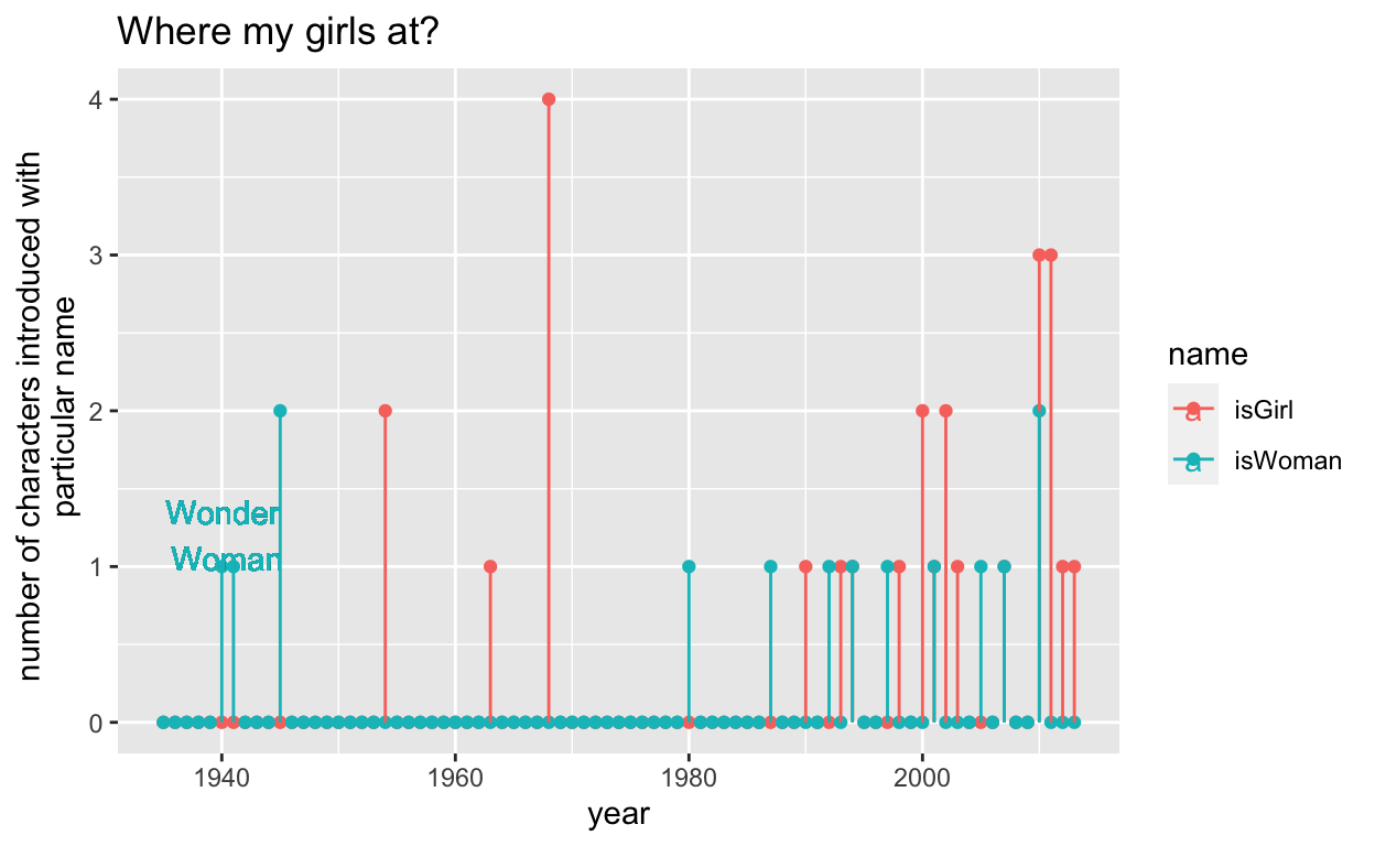
[1] 0

sub <- byYear[, c("year", "isGirl", "isWoman")]
toPlotUpdated <- sub %>% gather(name, value, -year)

ggplot(toPlotUpdated, aes(x = year, y = value, col = name)) +
  geom_point() +
  geom_segment(aes(x = year, y = 0, xend = year, yend = value, col = name)) +
  ylab("number of characters introduced with \n particular name") +
  ggtitle("Where my girls at?") +
  geom_text(aes(x = 1940.1, y = 1.2, label = "Wonder\n Woman"))

sub <- byYear[, c("year", "isBoy", "isMan")]
toPlotUpdated <- sub %>% gather(name, value, -year)

ggplot(toPlotUpdated, aes(x = year, y = value, col = name)) +
  geom_point() +
  geom_segment(aes(x = year, y = 0, xend = year, yend = value, col = name)) +
  ylab("number of characters introduced with \n particular name") +
  ggtitle("It's a man's (super) world") +
  geom_text(aes(x = 1986, y = 15, label = "Superman"))

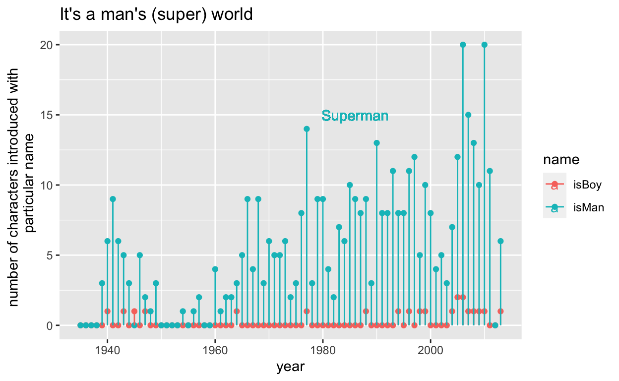
Take-Away: There are way more “men” than “boys” but “girl” is pervasive even after the Wonder Woman precedent.

Good v. Bad

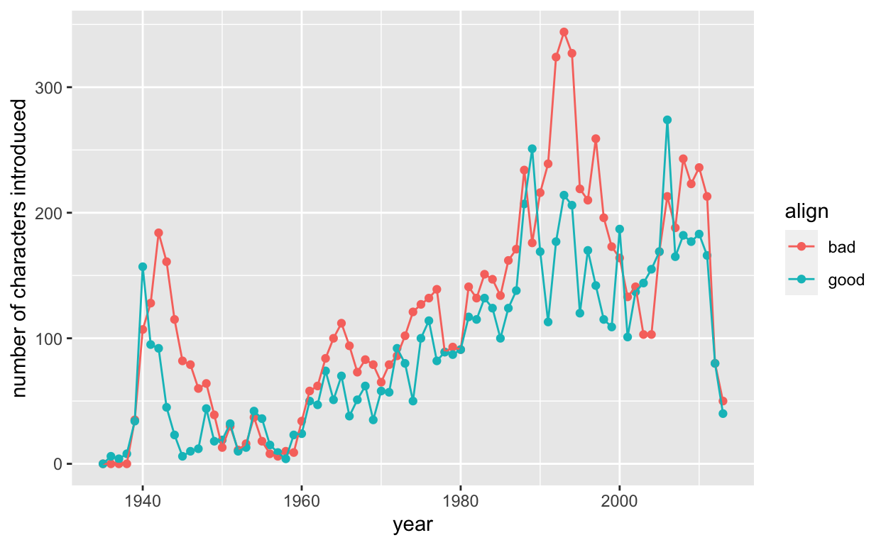
toPlot2 <- cb %>%
  group_by(year) %>%
  summarise(bad = length(which(align == "Bad Characters")), good = length(which(align == "Good Characters")))

toPlot2Update <- gather(toPlot2, align, count, -year)

ggplot(toPlot2Update, aes(x = year, y = count, col = align, group = align)) +
  geom_point() +
  geom_line() +
  ylab("number of characters introduced")

ggplot(toPlot2, aes(x = year, y = bad / good)) +
  geom_point() +
  geom_hline(yintercept = 1) +
  geom_text(aes(x = 1943, y = 10, label = "WWII")) +
  ggtitle("A hero(ine) can punch above their weight")

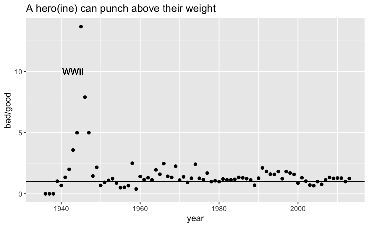
Take-Away: More bad than good characters are introduced over time fairly consistently. Interestingly, there is a peak in bad characters during World War II. Overall, it looks like each hero can handle more than one villain.

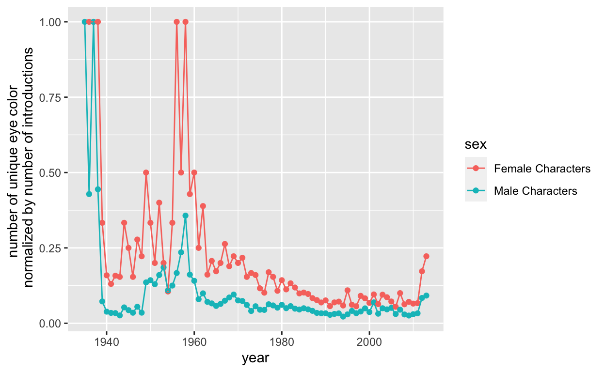
Appearance Variability

toPlot <- cb %>%
  group_by(year, sex) %>%
  summarise(count = n(), uniqueEye = length(unique(eye)) / n(), uniqueHair = length(unique(hair)) / n()) %>%
  filter(!is.na(sex)) %>%
  filter(sex %in% c("Male Characters", "Female Characters"))

ggplot(toPlot, aes(x = year, y = uniqueEye, col = sex, group = sex)) +
  geom_point() +
  geom_line() +
  ylab("number of unique eye color \n normalized by number of introductions")

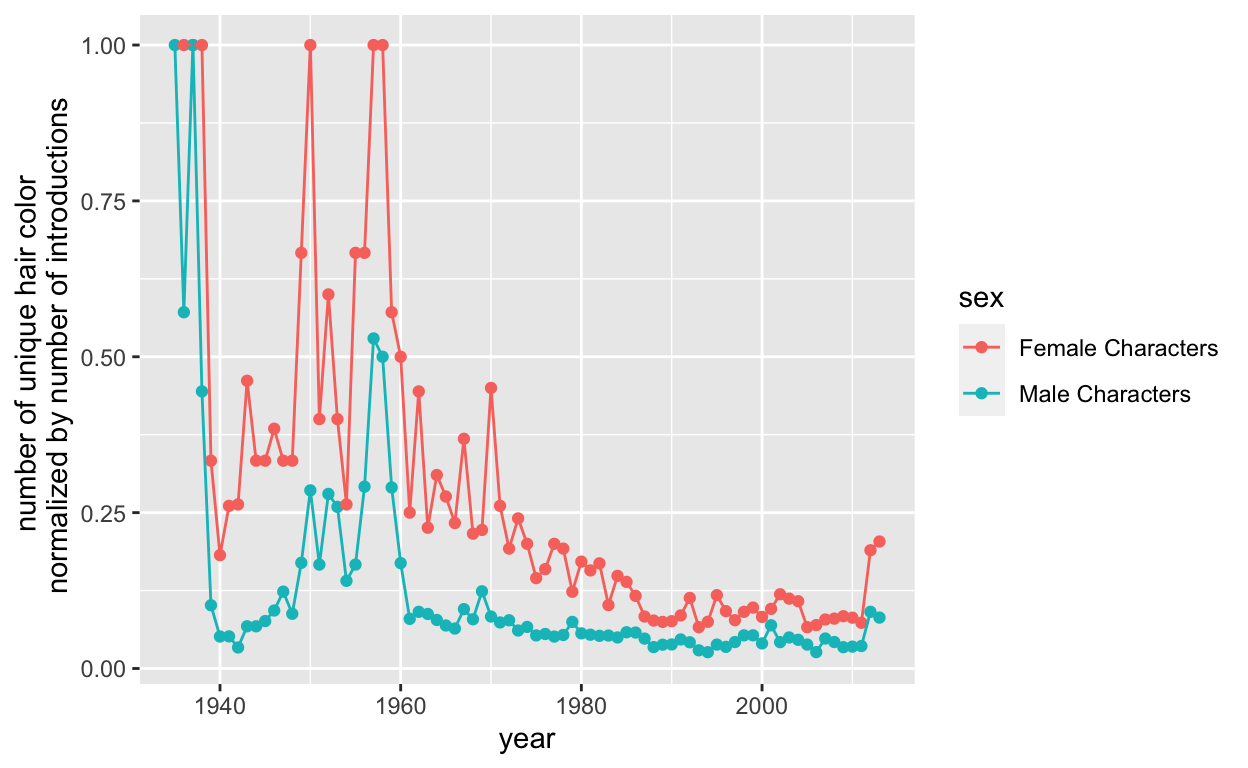
ggplot(toPlot, aes(x = year, y = uniqueHair, col = sex, group = sex)) +
  geom_point() +
  geom_line() +
  ylab("number of unique hair color \n normalized by number of introductions")

ggplot(toPlot, aes(x = year, y = count, col = sex, group = sex)) +
  geom_point() +
  geom_line() +
  ylab("number of introductions")

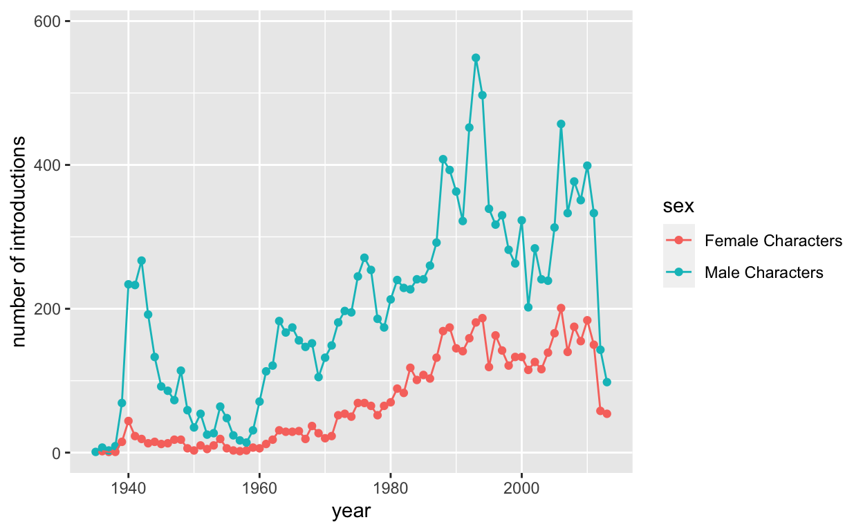
Take-Away: There is (proportionally) more variability in hair and eye color for female characters. There is a decline in variability in hair and eye color over time, but at least part of this is due to the rise in new characters (and a limit on the number of hair/eye colors).

Identity by Sex

bySex <- cb %>%
  group_by(sex) %>%
  summarise(count = n())

bySexID <- cb %>%
  group_by(sex, id) %>%
  summarise(count = n()) %>%
  inner_join(bySex, by = c("sex" = "sex")) %>%
  mutate(percent = count.x / count.y)

toPlot <- bySexID %>%
  filter(id %in% c("Public Identity", "Secret Identity", "No Dual Identity")) %>%
  filter(!is.na(sex))

toPlot2 <- as.data.frame(toPlot %>% arrange(sex))

ggplot(toPlot2, aes(id, y = percent, fill = sex)) +
  geom_bar(stat = "identity", position = position_dodge2(preserve = "total")) +
  theme(axis.text.x = element_text(angle = 45, hjust = 1))

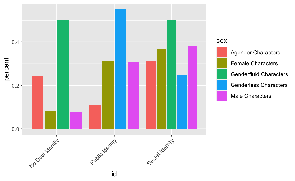
Take-Away: There doesn’t seem to be any real difference between female and men in terms of identity. I am reluctant to make any claims about the other categories because of their small sample size.