Let’s see how basic sentiment analysis classifies these Christmas hits. Luckily, I already have this code ready to go from my R Ladies Lightning Talk.
Top 5 Most Positive Songs (on average across lyric lines)
tt <- lyrics2 %>%
  group_by(track_title) %>%
  summarise(meanSentiment = mean(sentiment)) %>%
  arrange(desc(meanSentiment)) %>%
  head(5)

kable(tt) %>% kable_styling()
| track_title | meanSentiment |
|---|---|
| Silent Night | 0.6897360 |
| Sing Noel | 0.5814179 |
| God Rest Ye Merry Gentlemen | 0.3192399 |
| Hark! The Herald Angels Sing | 0.2859315 |
| O Holy Night | 0.2756963 |

Top 5 Most Negative Songs (on average across lyric lines)
tt <- lyrics2 %>%
  group_by(track_title) %>%
  summarise(meanSentiment = mean(sentiment)) %>%
  arrange(meanSentiment) %>%
  head(5)

kable(tt) %>% kable_styling()
| track_title | meanSentiment |
|---|---|
| You’re A Mean One, Mr. Grinch | -0.1200570 |
| This Cold War With You | -0.0752970 |
| To Each His Own | -0.0490823 |
| Come On Into My Arms | -0.0465882 |
| I’ll Break Out Again Tonight | -0.0404023 |

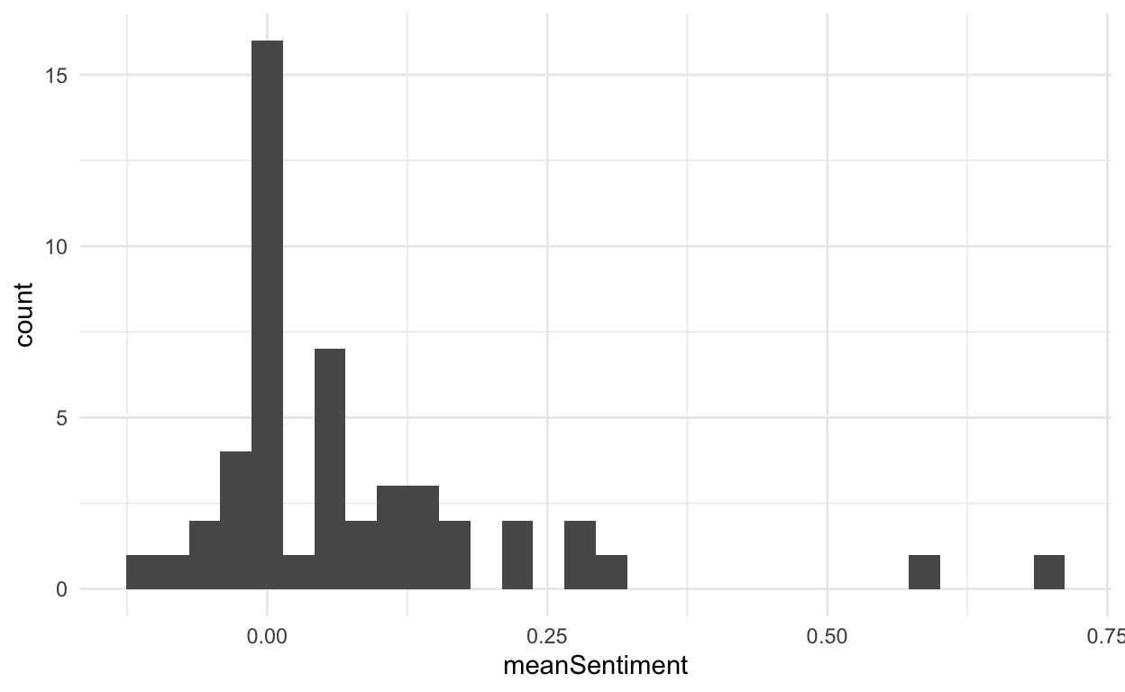
Distribution of Sentiment
There is a big peak at zero and then plenty of positive sentiment songs, but I would have expected more. However, this is just some basic analysis, so a more sophisticated approach might yield more like we expect.
lyrics3 <- lyrics2 %>%
  group_by(track_title) %>%
  summarise(meanSentiment = mean(sentiment))

ggplot(lyrics3, aes(meanSentiment)) +
  geom_histogram() +
  theme_minimal()
What makes Mr. Grinch so negative?
tt <- lyrics2 %>%
  filter(track_title == "You're A Mean One, Mr. Grinch") %>%
  select(sentiment, lyric) %>%
  arrange(sentiment) %>%
  head(5)

kable(tt) %>% kable_styling()
| sentiment | lyric |
|---|---|
| -0.5833333 | You’re a bad banana with a greasy black peel |
| -0.5833333 | You’re a bad banana with a greasy black peel |
| -0.4472136 | You’re a nasty, wasty skunk |
| -0.4472136 | You nauseate me, Mr. Grinch |
| -0.4472136 | You’re a crooked, jerky jocky |

What makes “Silent Night” so positive? Repetition! Free idea: analyze the repetition of the holiday hits.
tt <- lyrics2 %>%
  filter(track_title == "Silent Night") %>%
  select(sentiment, lyric) %>%
  arrange(desc(sentiment)) %>%
  head(5)

kable(tt) %>% kable_styling()
| sentiment | lyric |
|---|---|
| 1.06066 | Sleep in heavenly peace, sleep in heavenly peace |
| 1.06066 | Sleep in heavenly peace, sleep in heavenly peace |
| 1.06066 | Sleep in heavenly peace, sleep in heavenly peace |
| 1.06066 | Sleep in heavenly peace, sleep in heavenly peace |
| 1.06066 | Sleep in heavenly peace, sleep in heavenly peace |
Now let’s compare these songs to the songs on the Stoudt Christmas CD. This CD was lovingly curated by my dad, and I have listened to it every Christmas that I can remember, from in the car driving across Pennsylvania to see family to while decorating the tree. This year I don’t get to hear it played from the real CD at home, so I had to make a Spotify version. Check it out here. Usually I’m all for a good shuffled playlist, but this one has to be listened to in order, because TRADITION.
As soon as I hear those opening lines of Paul McCartney’s “Wonderful Christmastime” I know it’s holiday time!
blogdown::shortcode("youtube", "94Ye-3C1FC8")
{{% youtube "94Ye-3C1FC8" %}}
spotify_client_id <- "" ## put yours here
spotify_client_secret <- "" ## put yours here
access_token <- get_spotify_access_token(client_id = spotify_client_id, client_secret = spotify_client_secret)
stoudtChristmas <- get_playlist_tracks("0bso6lvKInn3myZ65vCSyj", authorization = access_token)
safe_lyrics <- safely(genius_lyrics)

artists <- unlist(lapply(stoudtChristmas$track.artists, function(x) {
  x[1, "name"]
}))
track_name <- stoudtChristmas$track.name

lyricsStoudt <- mapply(safe_lyrics, artists, track_name, SIMPLIFY = F)

didItWork <- lapply(lyricsStoudt, function(x) {
  x$error
})

sum(unlist(lapply(didItWork, is.null))) ## 14 of 21 have lyrics
setwd("~/Desktop/tidytuesday/week52_2019")
save(lyricsStoudt, file = "lyricsStoudtChristmas.RData")
Unfortunately, this Bruce classic got dropped.
blogdown::shortcode("youtube", "76WFkKp8Tjs")
{{% youtube "76WFkKp8Tjs" %}}
setwd("~/Desktop/tidytuesday/week52_2019")
load(file = "lyricsStoudtChristmas.RData")

test <- lapply(lyricsStoudt, function(x) {
  x$result
})

allL <- do.call("rbind", test)

allSentiment <- sentiment(allL$lyric)

allL$id <- 1:nrow(allL)

allL2 <- merge(allSentiment, allL, by.x = "element_id", by.y = "id")
Top 5 Most Positive Songs (on average across lyric lines)
tt <- allL2 %>%
  group_by(track_title) %>%
  summarise(meanSentiment = mean(sentiment)) %>%
  arrange(desc(meanSentiment)) %>%
  head(5)

kable(tt) %>% kable_styling()
| track_title | meanSentiment |
|---|---|
| Peace On Earth / Little Drummer Boy | 0.2620499 |
| Christmas Wrapping | 0.2461397 |
| Feliz Navidad | 0.2355009 |
| Rockin’ Around the Christmas Tree | 0.1862966 |
| White Christmas | 0.1810358 |
Top 5 Most Negative Songs (on average across lyric lines)
tt <- allL2 %>%
  group_by(track_title) %>%
  summarise(meanSentiment = mean(sentiment)) %>%
  arrange(meanSentiment) %>%
  head(5)

kable(tt) %>% kable_styling()
| track_title | meanSentiment |
|---|---|
| Blue Christmas | 0.0289615 |
| Jingle Bell Rock | 0.0459830 |
| Snoopy’s Christmas | 0.0695365 |
| I Saw Three Ships | 0.0697308 |
| I Saw Mommy Kissing Santa Claus | 0.0698132 |
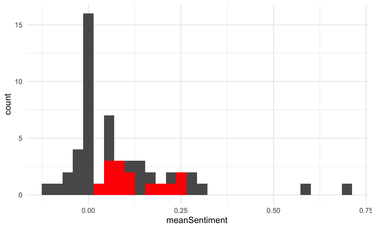
How does the Stoudt family Christmas album compare? We’re pretty positive (in red) in comparison to all of the hits.
allL3 <- allL2 %>%
  group_by(track_title) %>%
  summarise(meanSentiment = mean(sentiment))

ggplot(lyrics3, aes(meanSentiment)) +
  geom_histogram() +
  theme_minimal() +
  geom_histogram(data = allL3, aes(meanSentiment), fill = "red")
Happy Holidays!