Week 4 - Gender differences in Australian Average Taxable Income

RAW DATA
Article
DataSource: data.gov.au

Disparities in STEM

Take-aways

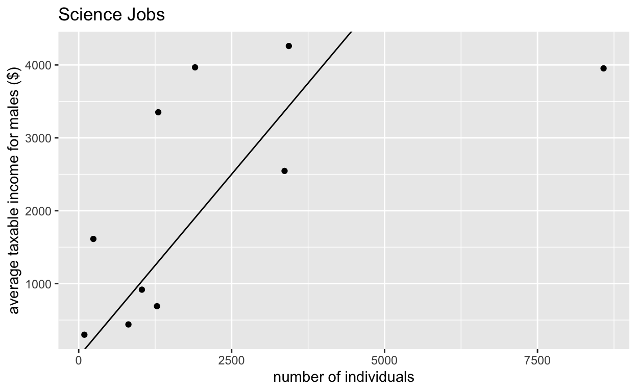
About equal number of indivuals in scientist jobs.
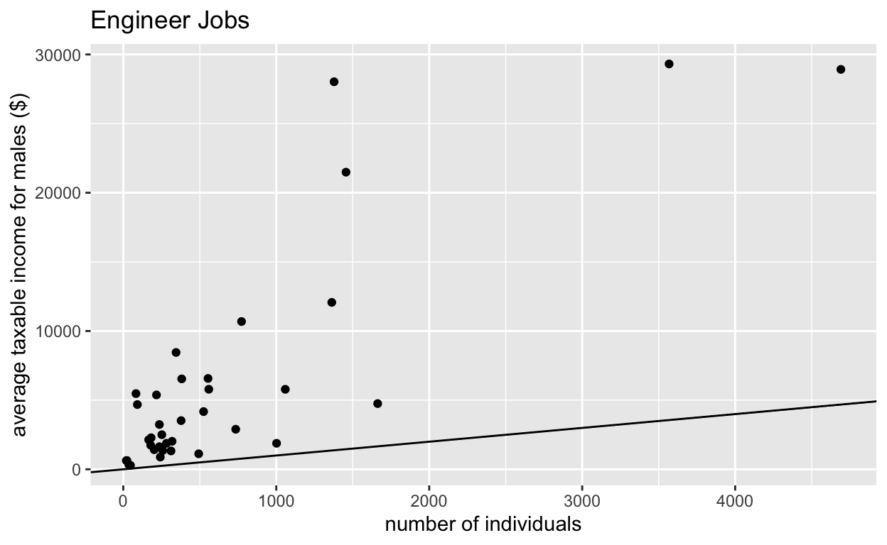
Many more males in engineering jobs.

(to be fair, should look into proportion of work force)

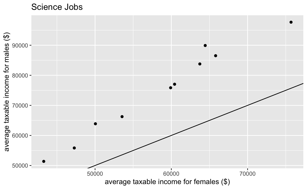
Rough OLS interpretation: For every dollar a woman makes in science, a man makes $1.52.
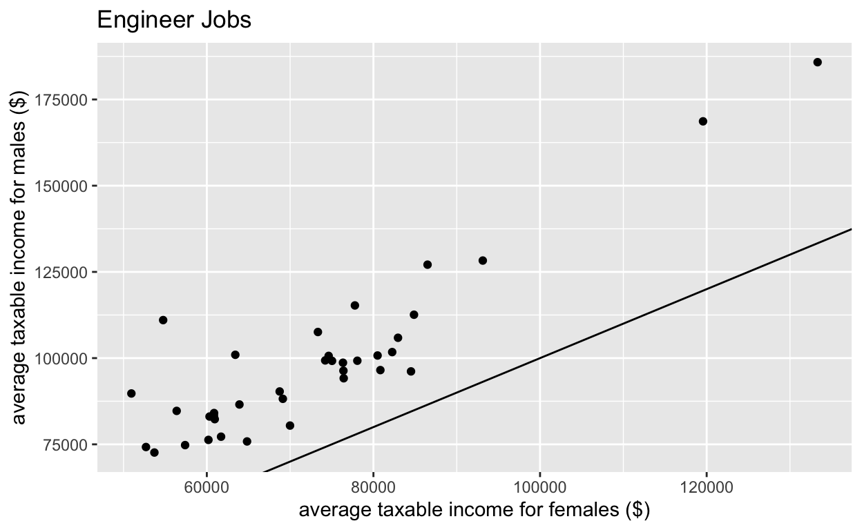
Rough OLS interpretation: For every dollar a woman makes in engineering, a man makes $1.26.

setwd("~/Desktop/tidytuesday/data/2018/2018-04-23")
aus <- read.csv("week4_australian_salary.csv")

require(ggplot2)
require(plotly) ## use to hover and see the job names

Look for STEM jobs.

aus[grep("stat", aus$occupation), ] ## looking for statistics

        X gender_rank                                  occupation
1131 1131         907 Garage attendant; Service station attendant
1132 1132         979 Garage attendant; Service station attendant
1786 1786         170                     Railway station manager
1787 1787         174                     Railway station manager
1792 1792         250                  Real estate agency manager
1793 1793         111                  Real estate agency manager
1794 1794         305                           Real estate agent
1795 1795         239                           Real estate agent
1796 1796         538                Real estate property manager
1797 1797         210                Real estate property manager
1994 1994         385                     Stock and station agent
1995 1995         457                     Stock and station agent
     gender individuals average_taxable_income
1131 Female        2434                  31906
1132   Male        2678                  34126
1786 Female         196                  74737
1787   Male        1220                  97952
1792 Female        2326                  66271
1793   Male        2437                 110559
1794 Female        6997                  62056
1795   Male       10983                  88045
1796 Female       18088                  49080
1797   Male        6708                  92500
1994 Female         108                  57899
1995   Male        1204                  67675

aus[grep("math", aus$occupation), ] ## nope

[1] X                      gender_rank           
[3] occupation             gender                
[5] individuals            average_taxable_income
<0 rows> (or 0-length row.names)

scientist <- aus[grep("scien", aus$occupation), ] ## bingo
engineer <- aus[grep("engineer", aus$occupation), ]

Get things organized. Not particularly tidy, but bear with me.

scientistG <- split(scientist, scientist$gender)
engineerG <- split(engineer, engineer$gender)

names(scientistG[[1]]) <- paste("F", names(scientistG[[1]]), sep = "")
names(scientistG[[2]]) <- paste("M", names(scientistG[[2]]), sep = "")

names(engineerG[[1]]) <- paste("F", names(engineerG[[1]]), sep = "")
names(engineerG[[2]]) <- paste("M", names(engineerG[[2]]), sep = "")

scientistFull <- cbind(scientistG[[1]], scientistG[[2]])
engineerFull <- cbind(engineerG[[1]], engineerG[[2]])

Look at number of individuals in each job

The line is y=x. If there was gender parity, we would see points lying around this line. You can hover to see the job titles.

p <- ggplot(scientistFull, aes(x = Findividuals, y = Mindividuals, text = Moccupation)) +
  geom_point() +
  geom_abline(intercept = 0, slope = 1) +
  xlab("number of individuals") +
  ylab("average taxable income for males ($)") +
  ggtitle("Science Jobs")
p ## for static version on github

p <- ggplotly(p)
p

p <- ggplot(engineerFull, aes(x = Findividuals, y = Mindividuals, text = Moccupation)) +
  geom_point() +
  geom_abline(intercept = 0, slope = 1) +
  xlab("number of individuals") +
  ylab("average taxable income for males ($)") +
  ggtitle("Engineer Jobs")
p ## for static version on github

p <- ggplotly(p)
p

Look at salary

Again the line is y=x. If there was gender parity, we would see points lying around this line. You can hover to see the job titles.

p <- ggplot(scientistFull, aes(x = Faverage_taxable_income, y = Maverage_taxable_income, text = Moccupation)) +
  geom_point() +
  geom_abline(intercept = 0, slope = 1) +
  xlab("average taxable income for females ($)") +
  ylab("average taxable income for males ($)") +
  ggtitle("Science Jobs")
p ## for static version on github

# p <- ggplotly(p) ## to look at job titles
# p

p <- ggplot(engineerFull, aes(x = Faverage_taxable_income, y = Maverage_taxable_income, text = Moccupation)) +
  geom_point() +
  geom_abline(intercept = 0, slope = 1) +
  xlab("average taxable income for females ($)") +
  ylab("average taxable income for males ($)") +
  ggtitle("Engineer Jobs")
p ## for static version on github

# p <- ggplotly(p) ## to look at job titles
# p

Rough Modeling

lm(scientistG[[2]]$Maverage_taxable_income ~ scientistG[[1]]$Faverage_taxable_income)


Call:
lm(formula = scientistG[[2]]$Maverage_taxable_income ~ scientistG[[1]]$Faverage_taxable_income)

Coefficients:
                            (Intercept)  
                             -14063.862  
scientistG[[1]]$Faverage_taxable_income  
                                  1.521

lm(engineerG[[2]]$Maverage_taxable_income ~ engineerG[[1]]$Faverage_taxable_income)


Call:
lm(formula = engineerG[[2]]$Maverage_taxable_income ~ engineerG[[1]]$Faverage_taxable_income)

Coefficients:
                           (Intercept)  
                              6543.508  
engineerG[[1]]$Faverage_taxable_income  
                                 1.261

Australian Salaries by Gender